Introduction

Data Analysis and Classification on a subset of data about polls for the 2006 and 2010 elections in Brazil for the “Câmara Federal de Deputados”. Data was taken from the TSE portal which originally encompassed approximately 7300 candidates.

Data Overview

The variables

The response variable is the variable that you are interested in reaching conclusions about.

A predictor variable is a variable used to predict another variable.

Our response variable will be "situacao", we want to study how well the predictor variables can help predict its behavior and how they impact in the linear regression.

Each item corresponds to a candidate, the attributes of each item are as follows:

ano : Year at which the election took place.
sequencial_candidato : Sequential ID to map the candidates
nome : Name of the candidate
uf : Federate state to which the candidate belongs.
partido : Political party to which the candidate belongs.
quantidade_doacoes : Number of donations received during political campaign.
quantidade_doadores : Number of donors that contributed to the candidate’s political campaign.
total_receita : Total revenue.
media_receita : Mean revenue.
recursos_de_outros_candidatos.comites : Revenue from other candidate’s committees.
recursos_de_pessoas_fisicas : Revenue from individuals.
recursos_de_pessoas_juridicas : Revenue from legal entities.
recursos_proprios : Revenue from personal resources.
recursos_de_partido_politico : Revenue from political party.
quantidade_despesas : Number of expenses.
quantidade_fornecedores : Number of suppliers.
total_despesa : Total expenditure.
media_despesa : Mean expenditure.
cargo : Position.
sexo : Sex.
grau : Level of education.
estado_civil : Marital status.
ocupacao : Candidate’s occupation up to the election.
situacao : Whether the candidate was elected.

Loading Data

readr::read_csv(here::here('evidences/train_class.csv'),
                progress = FALSE,
                local=readr::locale("br"),
                col_types = cols(ano = col_integer(),
                                 sequencial_candidato = col_character(),
                                 quantidade_doacoes = col_integer(),
                                 quantidade_doadores = col_integer(),
                                 total_receita = col_double(),
                                 media_receita = col_double(),
                                 recursos_de_outros_candidatos.comites = col_double(),
                                 recursos_de_pessoas_fisicas = col_double(),
                                 recursos_de_pessoas_juridicas = col_double(),
                                 recursos_proprios = col_double(),
                                 `recursos_de_partido_politico` = col_double(),
                                 quantidade_despesas = col_integer(),
                                 quantidade_fornecedores = col_integer(),
                                 total_despesa = col_double(),
                                 media_despesa = col_double(),
                                 situacao = col_character(),
                                 .default = col_character())) %>%
  mutate(sequencial_candidato = as.numeric(sequencial_candidato),
         estado_civil = as.factor(estado_civil),
         ocupacao = as.factor(ocupacao),
         situacao = as.factor(situacao),
         partido = as.factor(partido),
         grau = as.factor(grau),
         sexo = as.factor(sexo),
         uf = as.factor(uf)) -> data

data %>%
  glimpse()

## Observations: 7,622
## Variables: 24
## $ ano                                   <int> 2006, 2006, 2006, 2006, 20…
## $ sequencial_candidato                  <dbl> 10001, 10002, 10002, 10002…
## $ nome                                  <chr> "JOSÉ LUIZ NOGUEIRA DE SOU…
## $ uf                                    <fct> AP, RO, AP, MS, RO, AP, PI…
## $ partido                               <fct> PT, PT, PT, PRONA, PT, PT,…
## $ quantidade_doacoes                    <int> 6, 13, 17, 6, 48, 8, 6, 14…
## $ quantidade_doadores                   <int> 6, 13, 16, 6, 48, 8, 6, 7,…
## $ total_receita                         <dbl> 16600.00, 22826.00, 158120…
## $ media_receita                         <dbl> 2766.67, 1755.85, 9301.22,…
## $ recursos_de_outros_candidatos.comites <dbl> 0.00, 6625.00, 2250.00, 0.…
## $ recursos_de_pessoas_fisicas           <dbl> 9000.00, 15000.00, 34150.0…
## $ recursos_de_pessoas_juridicas         <dbl> 6300.00, 1000.00, 62220.80…
## $ recursos_proprios                     <dbl> 1300.00, 201.00, 59500.00,…
## $ recursos_de_partido_politico          <dbl> 0, 0, 0, 0, 0, 0, 0, 0, 0,…
## $ quantidade_despesas                   <int> 14, 24, 123, 8, 133, 38, 9…
## $ quantidade_fornecedores               <int> 14, 23, 108, 8, 120, 37, 9…
## $ total_despesa                         <dbl> 16583.60, 20325.99, 146011…
## $ media_despesa                         <dbl> 1184.54, 846.92, 1187.09, …
## $ cargo                                 <chr> "DEPUTADO FEDERAL", "DEPUT…
## $ sexo                                  <fct> MASCULINO, FEMININO, FEMIN…
## $ grau                                  <fct> ENSINO MÉDIO COMPLETO, SUP…
## $ estado_civil                          <fct> CASADO(A), SOLTEIRO(A), VI…
## $ ocupacao                              <fct> "VEREADOR", "SERVIDOR PÚBL…
## $ situacao                              <fct> nao_eleito, nao_eleito, el…

data %>%
  map_df(function(x) sum(is.na(x))) %>%
  gather(feature, num_nulls) %>%
  arrange(desc(num_nulls))

## # A tibble: 24 x 2
##    feature                               num_nulls
##    <chr>                                     <int>
##  1 ano                                           0
##  2 sequencial_candidato                          0
##  3 nome                                          0
##  4 uf                                            0
##  5 partido                                       0
##  6 quantidade_doacoes                            0
##  7 quantidade_doadores                           0
##  8 total_receita                                 0
##  9 media_receita                                 0
## 10 recursos_de_outros_candidatos.comites         0
## # … with 14 more rows

Data Exploration

Imbalance on class distribution

data %>%
  ggplot(aes(situacao)) +
  geom_bar() +
  labs(x="Situation", y="Absolute Frequency")

data %>%
  group_by(situacao) %>%
  summarise(num = n()) %>%
  ungroup() %>%
  mutate(total = sum(num),
         proportion = num/total)

## # A tibble: 2 x 4
##   situacao     num total proportion
##   <fct>      <int> <int>      <dbl>
## 1 eleito      1026  7622      0.135
## 2 nao_eleito  6596  7622      0.865

There’s a strong imbalance in the class distribution of the dataset with around 13% of the entries in the class “eleito” (elected).

This imbalance can lead to a bias in the model that will learn to overlook the less frequent classes. Such bias can have a negative impact in the model generalization and its performance.
- We can restore balance by removing instances from the most frequent class \(undersampling\).
- We can restore balance by adding instances from the most frequent class \(oversampling\).

data %>% 
  select(-ano,
         -sequencial_candidato,
         -nome) %>%
  select(
    quantidade_doacoes,
    quantidade_doadores,
    total_receita,
    media_receita,
    recursos_de_outros_candidatos.comites,
    recursos_de_pessoas_fisicas,
    recursos_de_pessoas_juridicas,
    recursos_proprios,
    `recursos_de_partido_politico`) %>%
  na.omit() %>%
  ggcorr(palette = "RdBu", label = TRUE,
       hjust = 0.95, label_size = 3,size = 3,
       nbreaks = 5, layout.exp = 5) +
  ggtitle("Correlation plot for employed variables")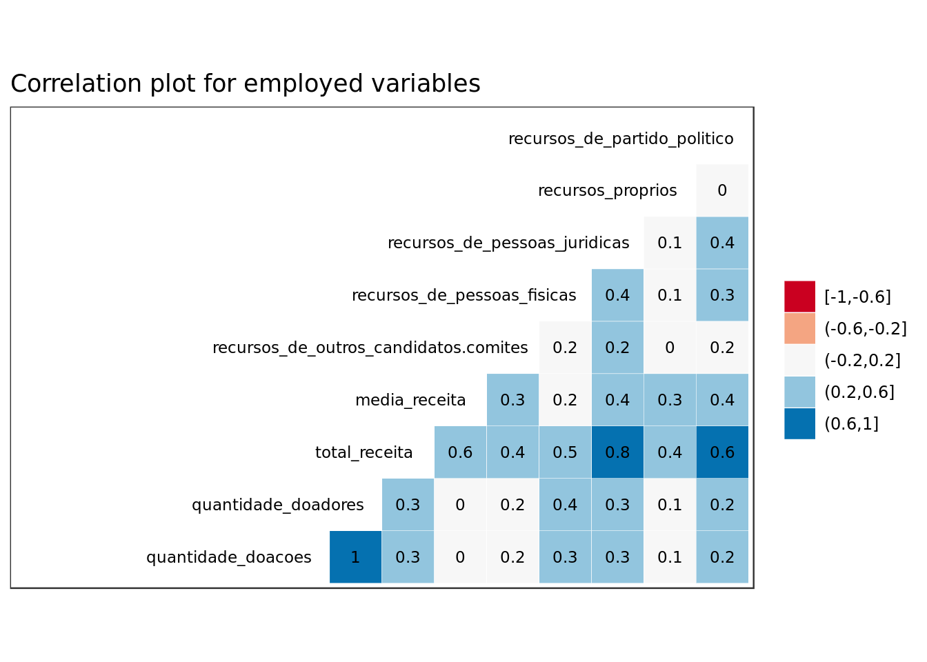

Predictors such as quantidade_doacoes (Number of Donations) and quantidade_doadores (Number of Donors) are highly correlated and therefore redundant.

data %>%
  ggplot(aes(situacao,recursos_proprios)) +
  geom_boxplot() + 
  coord_flip() +
  labs(y="Revenue from personal resources (R$)", x="Situation")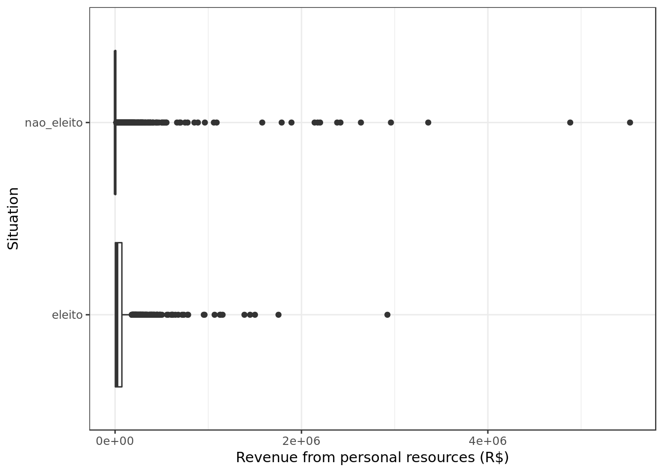

data %>%
  ggplot(aes(situacao,
             recursos_de_partido_politico)) +
  geom_boxplot() + 
  coord_flip() +
  labs(y="Revenue from political party. (R$)", x="Situation")

Candidates who were elected had overall more revenue form their political party

data %>%
  ggplot(aes(situacao,
             recursos_de_outros_candidatos.comites)) +
  geom_boxplot() + 
  coord_flip() +
  labs(y="Revenue from other candidate’s committees (R$)", x="Situation")

data %>%
  ggplot(aes(situacao,
             recursos_de_pessoas_fisicas)) +
  geom_boxplot() + 
  coord_flip() +
  labs(y="Revenue from individuals (R$)", x="Situation")

Candidates who were elected had overall more revenue form individuals.

data %>%
  ggplot(aes(situacao,
             recursos_de_pessoas_juridicas)) +
  geom_boxplot() + 
  coord_flip() +
  labs(y="Revenue from legal entities (R$)", x="Situation")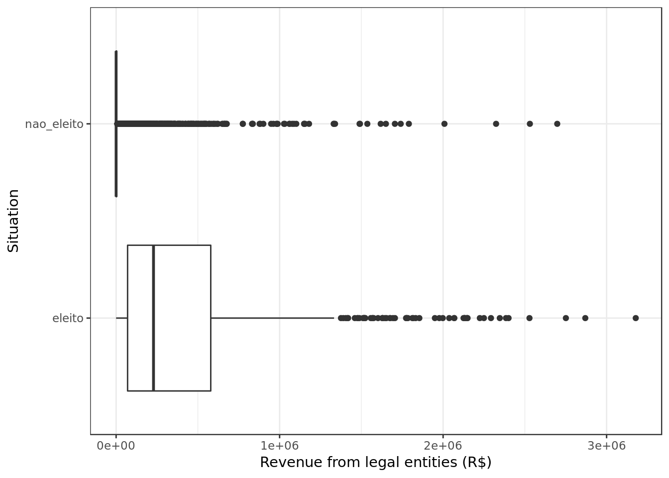

Financial support from legal entities (such as companies) seems to have been a game changer on whether a candidate was elected or not.

data %>%
  ggplot(aes(situacao,
             quantidade_doacoes)) +
  geom_boxplot() + 
  coord_flip() +
  labs(y="Number of donations", x="Situation")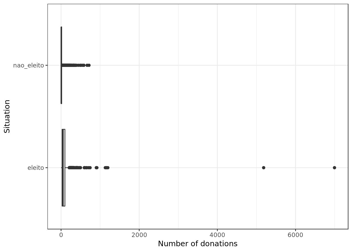

data %>%
  ggplot(aes(situacao,
             quantidade_doadores)) +
  geom_boxplot() + 
  coord_flip() +
  labs(y="Number of donators", x="Situation")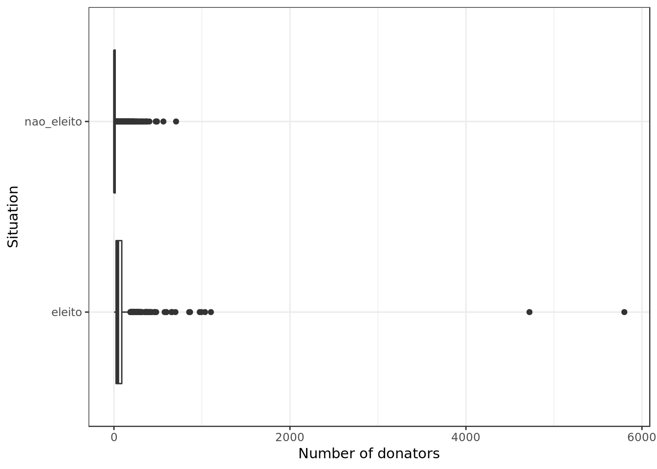

data %>%
  ggplot(aes(situacao,
             media_receita)) +
  geom_boxplot() + 
  coord_flip() +
  labs(y="Mean expenditure", x="Situation")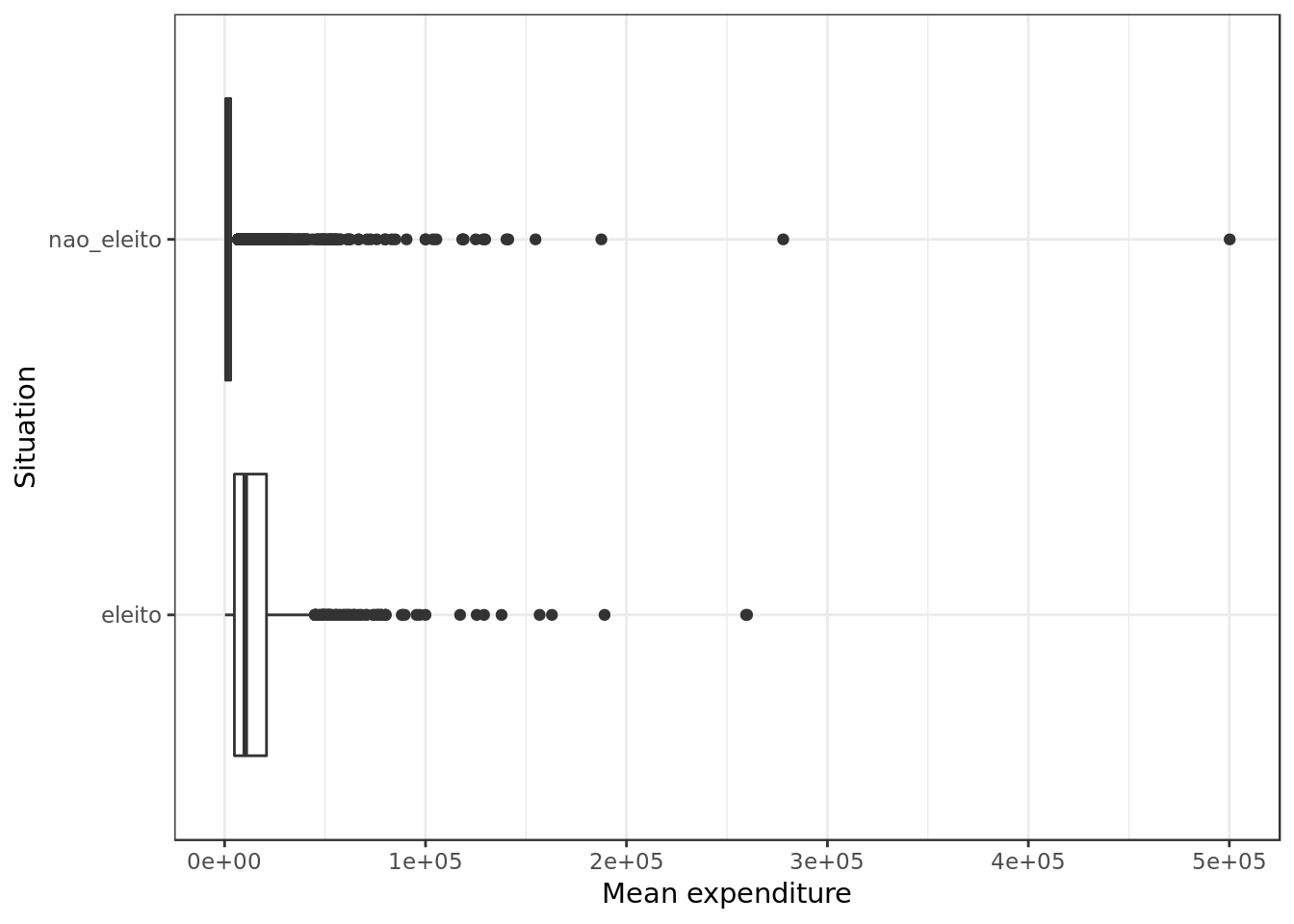

data %>%
  ggplot(aes(situacao,
             total_receita)) +
  geom_boxplot() + 
  coord_flip() +
  labs(y="Total expenditure", x="Situation")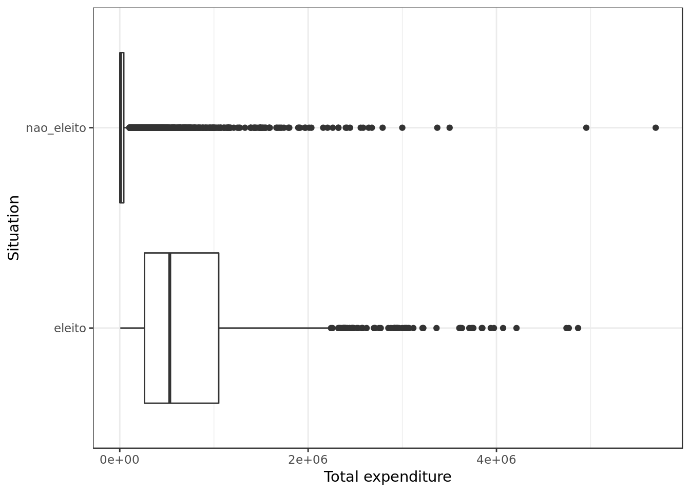

Who got elected spent a lot more, once again money seems to be the real gatekeeper.

data %>%
ggplot() +
   geom_mosaic(aes(x = product(sexo, situacao),
                   fill=sexo)) +
   theme(axis.title.y=element_blank(),
        axis.text.y=element_blank(),
        axis.ticks.y=element_blank()) +
  guides(fill = guide_legend(title = "Sex"))  +
  labs(x="Situation")

Relatively, we see more men being elected.

data %>%
ggplot() +
  geom_mosaic(aes(x = product(grau, situacao),
                   fill=grau)) +
  theme(axis.title.y=element_blank(),
        axis.text.y=element_blank(),
        axis.ticks.y=element_blank()) +
  guides(fill = guide_legend(title = "Level of education"))  +
  labs(x="Situation")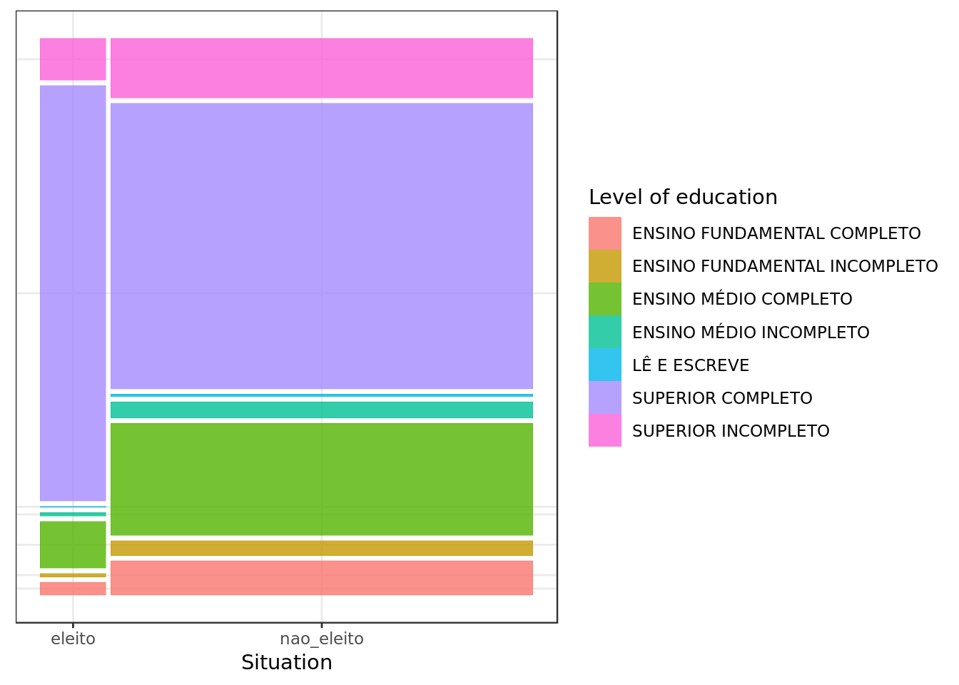

Those with a better level of education seem to have had the upper hand in the elections.

data %>%
ggplot() +
   geom_mosaic(aes(x = product(estado_civil, situacao),
                   fill=estado_civil)) +
   theme(axis.title.y=element_blank(),
        axis.text.y=element_blank(),
        axis.ticks.y=element_blank()) +
  guides(fill = guide_legend(title = "Marital Status"))  +
  labs(x="Situation")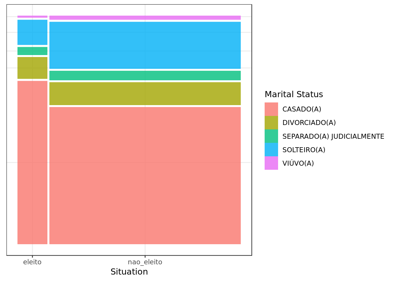

Relatively, married people are more likely to be elected in this group.

Preparing data

Splitting data

set.seed(107)

data$id <- 1:nrow(data)

data %>% 
  dplyr::sample_frac(.8) -> train

cat("#### Train Shape",
    "\n##### Observations: ",nrow(train),
    "\n##### Variables: ",ncol(train))

## #### Train Shape 
## ##### Observations:  6098 
## ##### Variables:  25

dplyr::anti_join(data, 
                 train, 
                 by = 'id') -> test

cat("#### Test Shape",
    "\n##### Observations: ",nrow(test),
    "\n##### Variables: ",ncol(test))

## #### Test Shape 
## ##### Observations:  1524 
## ##### Variables:  25

train %>%
    select(-ano,-nome,-id,-sequencial_candidato) -> train

test %>%
    select(-ano,-nome,-id,-sequencial_candidato) -> test

train %>%
  dplyr::select_if(.,is.numeric) -> train.numeric

train %>%
  dplyr::select_if(.,negate(is.numeric)) -> train.categorical

test %>%
  dplyr::select_if(.,is.numeric) -> test.numeric

test %>%
  dplyr::select_if(.,negate(is.numeric)) -> test.categorical

Scale and Center

train.numeric %>%
  preProcess(.,method = c("center","scale")) -> processParams

processParams %>%
  predict(.,train.numeric) -> train.numeric 

processParams %>% 
  predict(.,test.numeric) -> test.numeric 

processParams

## Created from 6098 samples and 13 variables
## 
## Pre-processing:
##   - centered (13)
##   - ignored (0)
##   - scaled (13)

One Hot Encoding

train.numeric %>%
  dplyr::bind_cols(train.categorical) -> train

test.numeric %>%
  dplyr::bind_cols(test.categorical) -> test

encoding <- build_encoding(dataSet = train,
                          cols = c("uf","sexo","grau","ocupacao",
                                   "partido","estado_civil"),
                          verbose = F)

train <- one_hot_encoder(dataSet = train,
                          encoding = encoding,
                          drop = TRUE,
                          verbose = F)

cat("#### Train Shape",
    "\n##### Observations: ",nrow(train),
    "\n##### Variables: ",ncol(train))

Train Shape

Observations: 6098

Variables: 263

test <- one_hot_encoder(dataSet = test,
                          encoding = encoding,
                          drop = TRUE,
                          verbose = F)

cat("#### Data Shape",
    "\n##### Observations: ",nrow(test),
    "\n##### Variables: ",ncol(test))

## #### Data Shape 
## ##### Observations:  1524 
## ##### Variables:  263

Near Zero Variance Predictors

train %>%
  nearZeroVar(saveMetrics = TRUE) %>%
  tibble::rownames_to_column("variable") %>%
  filter(nzv == T) %>% 
  pull(variable) -> near_zero_vars

train %>% 
    select(-one_of(near_zero_vars)) -> train

test %>%
    select(-one_of(near_zero_vars)) -> test


near_zero_vars %>% 
  glimpse()

##  chr [1:224] "cargo" "uf.AC" "uf.AL" "uf.AM" "uf.AP" "uf.BA" "uf.CE" ...

Unbalanced dataset

In this section we shall test the candidate models without applying any sort of undersampling or oversampling to the employed data

Logistic Regression

f1 <- function(data, lev = NULL, model = NULL) {
  f1_val <- F1_Score(y_pred = data$pred,
                     y_true = data$obs,
                     positive = lev[1])
  c(F1 = f1_val)
}

F_Measure <- function(expected, predicted, ...) {
  data.frame(expected=expected,
             prediction=predicted) %>%
      mutate(TP = ifelse(expected == "eleito" & 
                         prediction == "eleito",1,0),
             TN = ifelse(expected == "nao_eleito" &
                         prediction == "nao_eleito",1,0),
             FN = ifelse(expected == "eleito" &
                         prediction == "nao_eleito",1,0),
             FP = ifelse(expected == "nao_eleito" &
                         prediction == "eleito",1,0)) -> result
  result  %>%
    summarize(TP = sum(TP),
              TN = sum(TN),
              FP = sum(FP),
              FN = sum(FN)) %>%
    mutate(recall = TP / (TP + FN),
           precision = TP / (TP + FP),
           accuracy = (TP + TN)/(TP + TN + FP + FN),
           f_measure = 2 * (precision * recall) / (precision + recall)) -> result
  
  return(result)
}

rlGrid <- expand.grid( cost = c(200,2,0.02),
                       loss = c("L1", "L2_dual", "L2_primal"),
                       epsilon = c(0.001,0.01) )
train %>%
  caret::train(situacao ~ .,
               data= .,
               method = "regLogistic",
               metric = "F1",
               trControl = trainControl(method = "boot",
                                        classProbs = TRUE,
                                        summaryFunction = f1,
                                        savePredictions = "final"),
               tuneGrid = rlGrid) -> model.rl

model.rl

## Regularized Logistic Regression 
## 
## 6098 samples
##   38 predictors
##    2 classes: 'eleito', 'nao_eleito' 
## 
## No pre-processing
## Resampling: Bootstrapped (25 reps) 
## Summary of sample sizes: 6098, 6098, 6098, 6098, 6098, 6098, ... 
## Resampling results across tuning parameters:
## 
##   cost   loss       epsilon  F1       
##   2e-02  L1         0.001    0.5841929
##   2e-02  L1         0.010    0.5850193
##   2e-02  L2_dual    0.001    0.5994658
##   2e-02  L2_dual    0.010    0.5994658
##   2e-02  L2_primal  0.001    0.5994150
##   2e-02  L2_primal  0.010    0.6000753
##   2e+00  L1         0.001    0.6342838
##   2e+00  L1         0.010    0.6359184
##   2e+00  L2_dual    0.001    0.6333125
##   2e+00  L2_dual    0.010    0.6333125
##   2e+00  L2_primal  0.001    0.6332243
##   2e+00  L2_primal  0.010    0.6335837
##   2e+02  L1         0.001    0.6329757
##   2e+02  L1         0.010    0.6355253
##   2e+02  L2_dual    0.001    0.6445493
##   2e+02  L2_dual    0.010    0.6487011
##   2e+02  L2_primal  0.001    0.6330532
##   2e+02  L2_primal  0.010    0.6344372
## 
## F1 was used to select the optimal model using the largest value.
## The final values used for the model were cost = 200, loss = L2_dual
##  and epsilon = 0.01.

model.rl %$%
  results %>%
  mutate(cost=as.factor(cost)) %>%
  ggplot(aes(epsilon,F1,
             color=cost)) +
  geom_line() +
  geom_point() +
  labs(y= "F1 (Bootstrap)", x="Tolerance") +
  facet_wrap(. ~ loss, labeller = "label_both") +
  guides(color = guide_legend(title = "Cost")) +
  theme(axis.text.x = element_text(angle = 60, hjust = 1))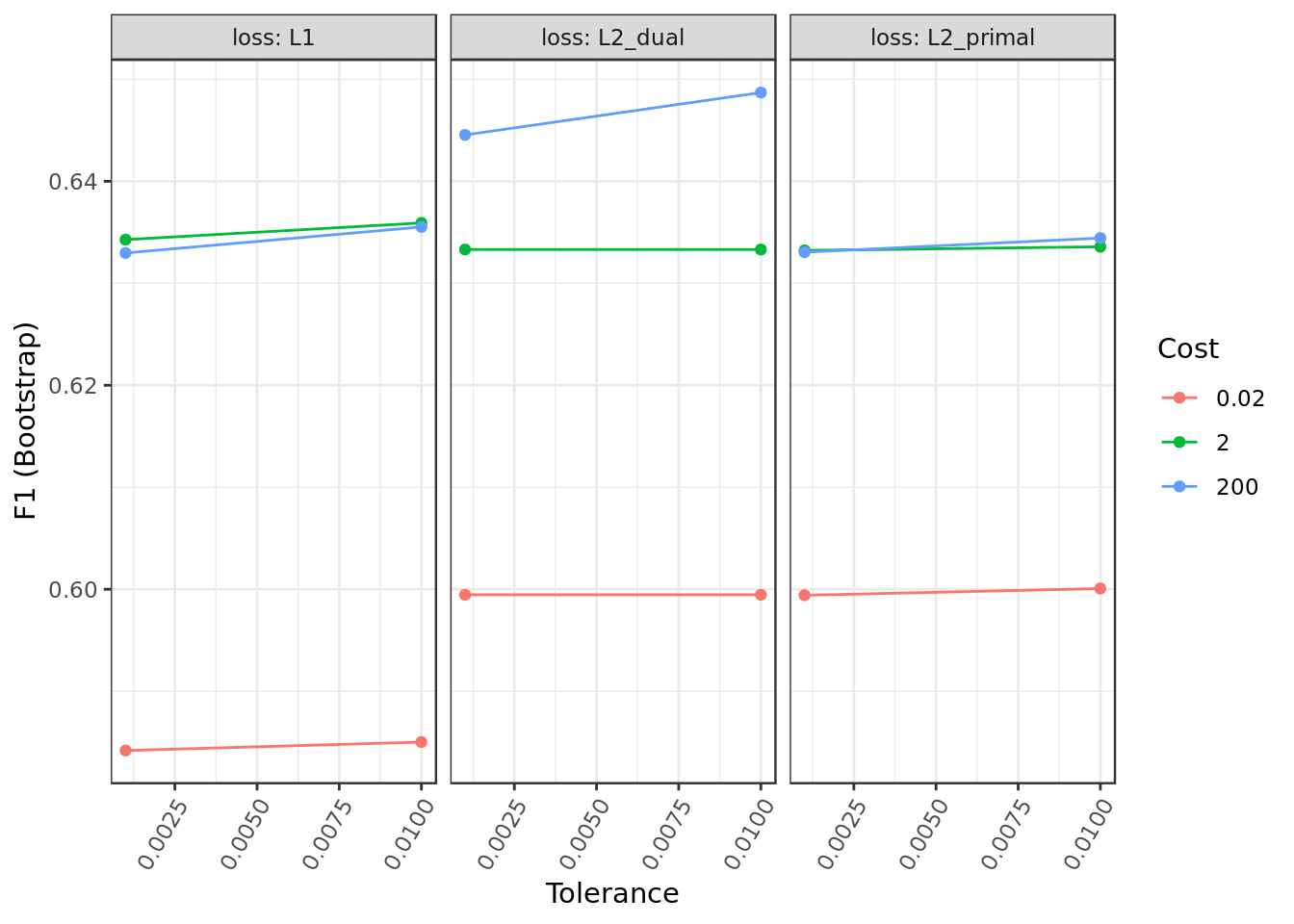

The hyper-parameter Loss seems to be the particularly meaningful for the Logistic Regression performance in this problem.

model.rl %>%
  varImp() %$%
  importance %>%
  as.data.frame() %>%
  rownames_to_column(var="Feature") %>%
  mutate(Feature = tolower(Feature)) %>%
  ggplot() +
  geom_col(aes(x = reorder(Feature,eleito),y = eleito),
           position = position_dodge(width=0.8),width=0.6) + 
  labs(x="Feature", y="Overall Importance") +
  coord_flip()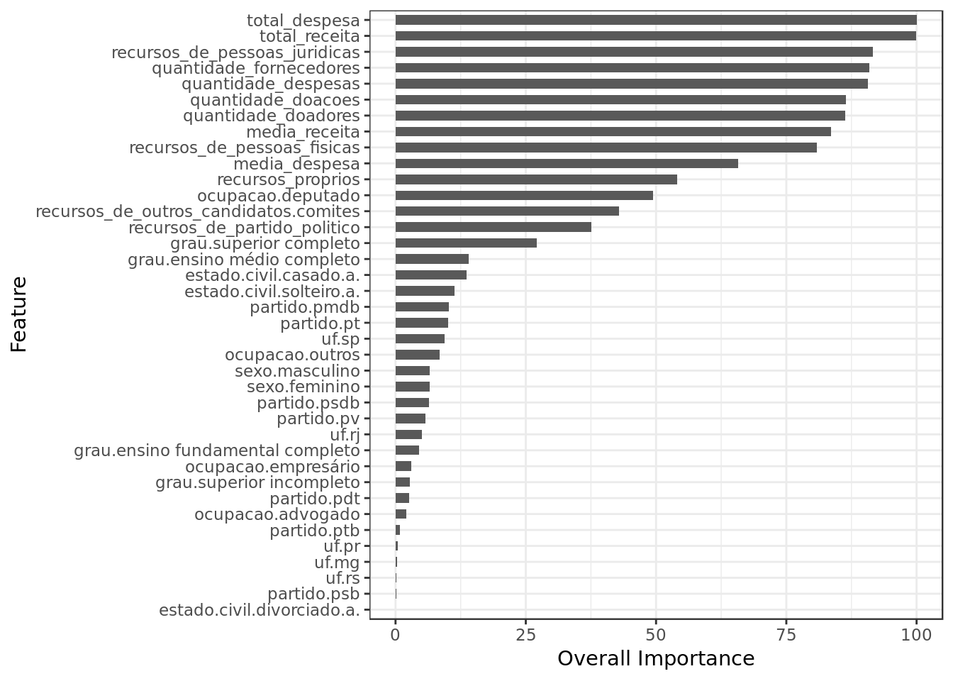

Total Receita (Total Revenue), Total Despesa (Total Expenditure) and Recursos de pessoas jurídicas (Revenue from Legal Entities) are together the three most important features in the model.
Despite regularization a lot of features were employed, however many were considered less important.

Quality metric

Train and Validation

model.rl %$% 
  pred %>% 
  F_Measure(expected = .$obs,
            predicted = .$pred)

##     TP    TN   FP   FN    recall precision  accuracy f_measure
## 1 4462 46905 1807 3006 0.5974826 0.7117563 0.9143289 0.6496324

A decent although uninspiring result.

Test

test %>%
  select(-situacao) %>%
  predict(object=model.rl,.) %>%
  F_Measure(test$situacao,.)

##    TP   TN FP FN    recall precision  accuracy f_measure
## 1 115 1268 43 98 0.5399061 0.7278481 0.9074803 0.6199461

The test result is rather close to the train/validation results, this is a good sign. However, the model results are not particularly promising.

K nearest neighbours

neighborsGrid <- expand.grid(.k = seq(from=1, to=50, by=1))

train %>%
  train(situacao ~ .,
        data = .,
        metric = "F1",
        method = "knn",
        na.action = na.omit,
        tuneGrid = neighborsGrid,
        trControl = trainControl(method = "boot",
                                 classProbs = TRUE,
                                 summaryFunction = f1,
                                 savePredictions = "final")) -> model.knn

model.knn

## k-Nearest Neighbors 
## 
## 6098 samples
##   38 predictors
##    2 classes: 'eleito', 'nao_eleito' 
## 
## No pre-processing
## Resampling: Bootstrapped (25 reps) 
## Summary of sample sizes: 6098, 6098, 6098, 6098, 6098, 6098, ... 
## Resampling results across tuning parameters:
## 
##   k   F1       
##    1  0.5824759
##    2  0.5875895
##    3  0.6007862
##    4  0.6061060
##    5  0.6144416
##    6  0.6200697
##    7  0.6241954
##    8  0.6311975
##    9  0.6356655
##   10  0.6336647
##   11  0.6366401
##   12  0.6399036
##   13  0.6392513
##   14  0.6434043
##   15  0.6464512
##   16  0.6462525
##   17  0.6458874
##   18  0.6491884
##   19  0.6477945
##   20  0.6480499
##   21  0.6472381
##   22  0.6445113
##   23  0.6465735
##   24  0.6457208
##   25  0.6461998
##   26  0.6482132
##   27  0.6486326
##   28  0.6496663
##   29  0.6500242
##   30  0.6499457
##   31  0.6499628
##   32  0.6509105
##   33  0.6506456
##   34  0.6504918
##   35  0.6509949
##   36  0.6496751
##   37  0.6487479
##   38  0.6485889
##   39  0.6476139
##   40  0.6484988
##   41  0.6487328
##   42  0.6487954
##   43  0.6478067
##   44  0.6501784
##   45  0.6495676
##   46  0.6487787
##   47  0.6490995
##   48  0.6492741
##   49  0.6478356
##   50  0.6486335
## 
## F1 was used to select the optimal model using the largest value.
## The final value used for the model was k = 35.

model.knn %$%
  bestTune %$% 
  k -> bestParameter

model.knn %$%
  results %>%
  ggplot(aes(k,F1)) +
  geom_vline(xintercept = bestParameter,
             color = "red") +
  geom_point(color="#0D98E8") +
  geom_line(color="#0D98E8") +
  labs(x="#Neighbors",
       y="F1 (Bootstrap)")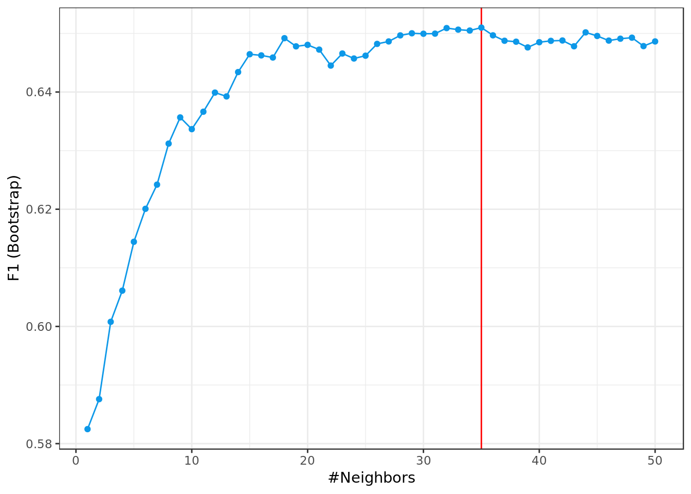

model.knn %>%
  varImp() %$%
  importance %>%
  as.data.frame() %>%
  rownames_to_column(var="Feature") %>%
  mutate(Feature = tolower(Feature)) %>%
  ggplot() +
  geom_col(aes(x = reorder(Feature,eleito),y = eleito),
           position = position_dodge(width=0.8),width=0.6) + 
  labs(x="Feature", y="Overall Importance") +
  coord_flip()

Total Receita (Total Revenue), Total Despesa (Total Expenditure) and Recursos de pessoas jurídicas (Revenue from Legal Entities) are together the three most important features in this model as well.
The KNN algorithm made use of almost all predictors, this may be a bad sign.

Quality metric

Train and Validation

model.knn %$% 
  pred %>% 
  F_Measure(expected = .$obs,
            predicted = .$pred)

##     TP    TN   FP   FN    recall precision  accuracy f_measure
## 1 4533 46832 2009 2845 0.6143941 0.6929074 0.9136591 0.6512931

Here we have slightly better results than those of the Logistic Regression.

Test

test %>%
  select(-situacao) %>%
  predict(object=model.knn,.) %>%
  F_Measure(test$situacao,.)

##    TP   TN FP FN  recall precision accuracy f_measure
## 1 122 1259 52 91 0.57277 0.7011494 0.906168  0.630491

We have modest results, but they are consonant with those from train/test.
- This suggests that the KNN model may be too simple for this particular instance, and bias would be the predominant component in the model error.

Decision Tree

rpart.grid <- expand.grid(.cp = seq(from=0, to=0.1, by=0.005))

caret::train(x = select(train, -situacao),
             y = train$situacao,
             metric = "F1",
             method = "rpart",
             na.action = na.omit,
             tuneGrid = rpart.grid,
             trControl = trainControl(method = "boot",
                                      classProbs = TRUE,
                                      summaryFunction = f1,
                                      savePredictions = "final")) -> model.tree

model.tree

## CART 
## 
## 6098 samples
##   38 predictors
##    2 classes: 'eleito', 'nao_eleito' 
## 
## No pre-processing
## Resampling: Bootstrapped (25 reps) 
## Summary of sample sizes: 6098, 6098, 6098, 6098, 6098, 6098, ... 
## Resampling results across tuning parameters:
## 
##   cp     F1       
##   0.000  0.6222605
##   0.005  0.6597754
##   0.010  0.6730765
##   0.015  0.6737400
##   0.020  0.6684035
##   0.025  0.6684085
##   0.030  0.6668214
##   0.035  0.6681258
##   0.040  0.6681258
##   0.045  0.6681258
##   0.050  0.6661671
##   0.055  0.6661671
##   0.060  0.6712018
##   0.065  0.6699034
##   0.070  0.6700850
##   0.075  0.6702300
##   0.080  0.6717618
##   0.085  0.6726706
##   0.090  0.6632295
##   0.095  0.6726590
##   0.100  0.6660222
## 
## F1 was used to select the optimal model using the largest value.
## The final value used for the model was cp = 0.015.

model.tree %$%
  bestTune %$% 
  cp -> bestParameter

model.tree %$%
  results %>%
  ggplot(aes(cp,F1)) +
  geom_vline(xintercept = bestParameter,
             color = "red") +
  geom_point(color="#0D98E8") +
  geom_line(color="#0D98E8") +
  labs(x="Complexity Parameter",
       y="F1 (Bootstrap)")

model.tree %$%
  finalModel %>%
  fancyRpartPlot(sub="")

The best performing tree seems simple yet reasonable.
- This tree may be in the border of an underfitting.

model.tree %>%
  varImp() %$%
  importance %>%
  as.data.frame() %>%
  rownames_to_column(var="Feature") %>%
  mutate(Feature = tolower(Feature)) %>%
  ggplot() +
  geom_col(aes(x = reorder(Feature,Overall),y = Overall),
           position = position_dodge(width=0.8),width=0.6) + 
  labs(x="Feature", y="Overall Importance") +
  coord_flip()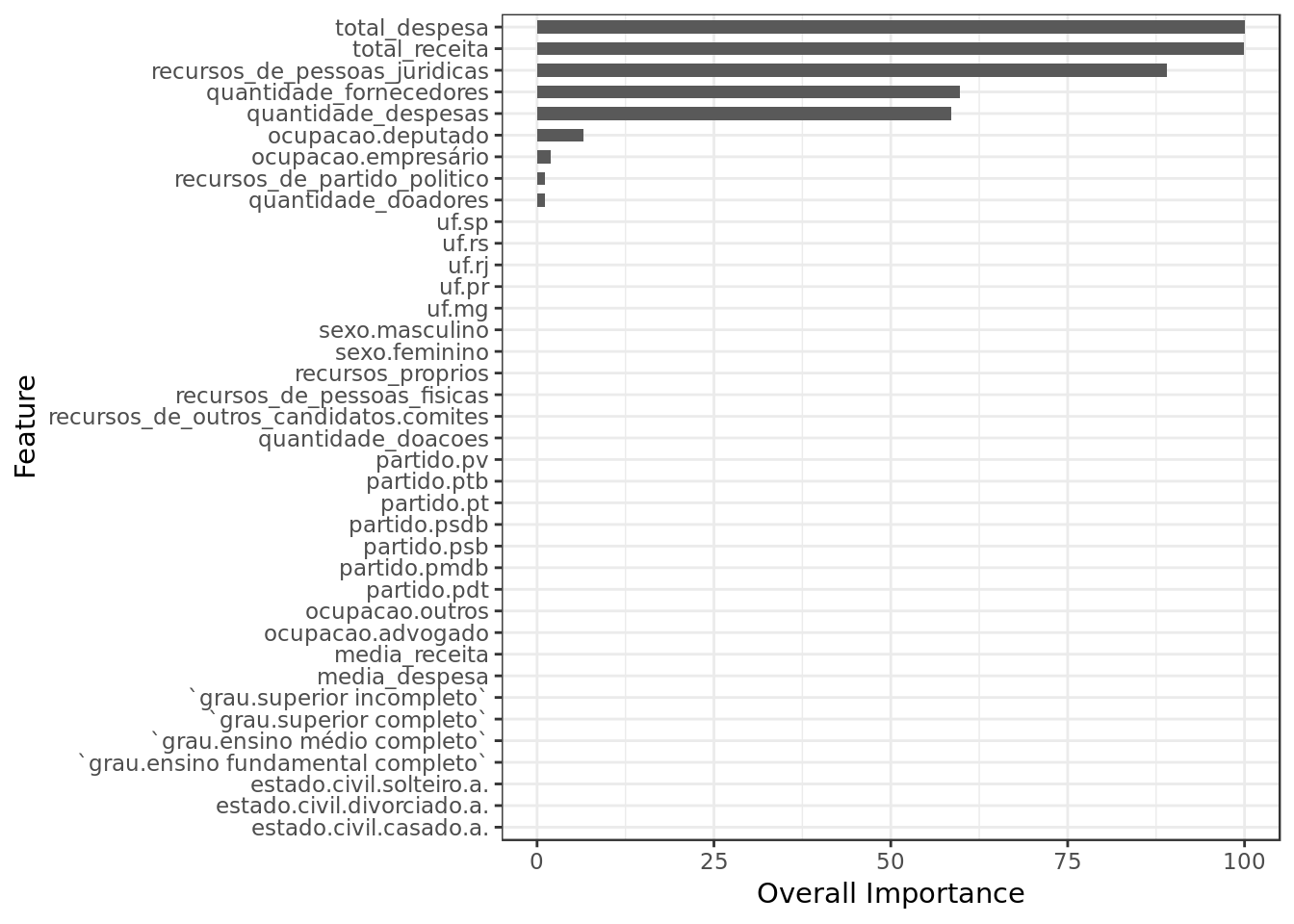

Total Receita (Total Revenue), Total Despesa (Total Expenditure) and Recursos de pessoas jurídicas (Revenue from Legal Entities) are together the three most important features in this model as well.
The tree used very few predictors which may indicate an underfitting, or simply that the tree captured the few meaningful predictors.

Quality metric

Train and Validation

model.tree %$% 
  pred %>% 
  F_Measure(expected = .$obs,
            predicted = .$pred)

##     TP    TN   FP   FN    recall precision  accuracy f_measure
## 1 4922 46495 2084 2667 0.6485703 0.7025407 0.9154145 0.6744776

Here we have surprisingly good results considering the simplicity of the tree.

Test

test %>%
  select(-situacao) %>%
  predict(object=model.tree,.) %>%
  F_Measure(test$situacao,.)

##    TP   TN FP FN   recall precision  accuracy f_measure
## 1 128 1252 59 85 0.600939  0.684492 0.9055118      0.64

We have slightly better results than those seen till now, on top of that they are consonant with those from train/test.

AdaBoost

train(x = select(train, -situacao),
      y = train$situacao,
      metric = "F1",
      na.action = na.exclude,
      method='adaboost',
      tuneLength=2,
      trControl = trainControl(savePredictions = "final",
                               summaryFunction = f1,
                               classProbs = TRUE,
                               method = "boot")) -> model.ada

model.ada

## AdaBoost Classification Trees 
## 
## 6098 samples
##   38 predictors
##    2 classes: 'eleito', 'nao_eleito' 
## 
## No pre-processing
## Resampling: Bootstrapped (25 reps) 
## Summary of sample sizes: 6098, 6098, 6098, 6098, 6098, 6098, ... 
## Resampling results across tuning parameters:
## 
##   nIter  method         F1       
##    50    Adaboost.M1    0.6634637
##    50    Real adaboost  0.6610069
##   100    Adaboost.M1    0.6645724
##   100    Real adaboost  0.6639414
## 
## F1 was used to select the optimal model using the largest value.
## The final values used for the model were nIter = 100 and method
##  = Adaboost.M1.

model.ada %$%
  results %>%
  ggplot(aes(nIter,F1, 
             color=as.factor(method))) +
  geom_point(shape=1) +
  geom_line() +
  labs(x="# Trees",y="F1 (Bootstrap)") +
  guides(color = guide_legend(title = "Method"))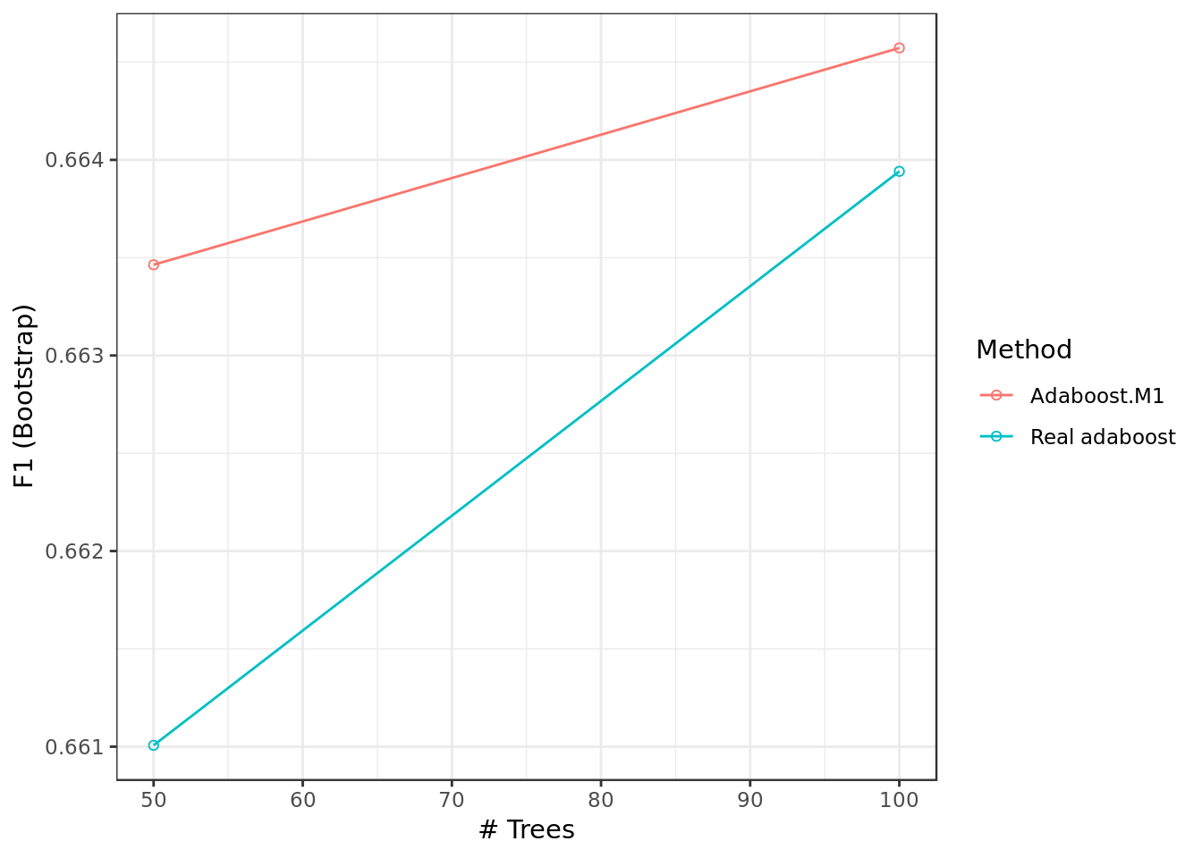

Train and Validation

model.ada %$% 
  pred %>% 
  F_Measure(expected = .$obs,
            predicted = .$pred)

##     TP    TN   FP   FN    recall precision  accuracy f_measure
## 1 4843 46233 2236 2644 0.6468545 0.6841362 0.9127886 0.6649732

Here we have better results than what we have seen so far.

Test

test %>%
  select(-situacao) %>%
  predict(object=model.ada,.) %>%
  F_Measure(test$situacao,.)

##    TP   TN FP FN    recall precision  accuracy f_measure
## 1 136 1250 61 77 0.6384977 0.6903553 0.9094488 0.6634146

The loss in the quality metric going from train/validation to test was small enough.
This suggest that the model did in fact fit the behavior of the problem and not noise.

Applying Oversample (SMOTE)

train %>%
  SMOTE(situacao ~ .,
        data = ., 
        perc.over = 200, 
        perc.under=200) -> oversampled

cat("#### Train Shape",
    "\n##### Observations: ",nrow(oversampled),
    "\n##### Variables: ",ncol(oversampled))

## #### Train Shape 
## ##### Observations:  5691 
## ##### Variables:  39

oversampled %>%
  group_by(situacao) %>%
  summarise(num = n()) %>%
  ungroup() %>%
  mutate(total = sum(num),
         proportion = num/total)

## # A tibble: 2 x 4
##   situacao     num total proportion
##   <fct>      <int> <int>      <dbl>
## 1 eleito      2439  5691      0.429
## 2 nao_eleito  3252  5691      0.571

BY means of SMOTE we have reduce the class imbalance considerably

Logistic Regression with SMOTE

rlGrid <- expand.grid( cost = c(0.02,0.1,2,20,100,200),
                       loss = c("L1", "L2_dual", "L2_primal"),
                       epsilon = seq(from=0.001,to=0.1, by=0.005) )
oversampled %>%
  caret::train(situacao ~ .,
               data= .,
               method = "regLogistic",
               metric = "F1",
               trControl = trainControl(method = "boot",
                                        classProbs = TRUE,
                                        summaryFunction = f1,
                                        savePredictions = "final"),
               tuneGrid = rlGrid) -> model.rl.smote

model.rl.smote

## Regularized Logistic Regression 
## 
## 5691 samples
##   38 predictors
##    2 classes: 'eleito', 'nao_eleito' 
## 
## No pre-processing
## Resampling: Bootstrapped (25 reps) 
## Summary of sample sizes: 5691, 5691, 5691, 5691, 5691, 5691, ... 
## Resampling results across tuning parameters:
## 
##   cost   loss       epsilon  F1       
##   2e-02  L1         0.001    0.8609407
##   2e-02  L1         0.006    0.8609313
##   2e-02  L1         0.011    0.8611976
##   2e-02  L1         0.016    0.8625802
##   2e-02  L1         0.021    0.8626373
##   2e-02  L1         0.026    0.8616010
##   2e-02  L1         0.031    0.8630162
##   2e-02  L1         0.036    0.8624694
##   2e-02  L1         0.041    0.8631067
##   2e-02  L1         0.046    0.8626822
##   2e-02  L1         0.051    0.8635124
##   2e-02  L1         0.056    0.8625129
##   2e-02  L1         0.061    0.8616411
##   2e-02  L1         0.066    0.8628480
##   2e-02  L1         0.071    0.8607301
##   2e-02  L1         0.076    0.8606394
##   2e-02  L1         0.081    0.8599239
##   2e-02  L1         0.086    0.8583560
##   2e-02  L1         0.091    0.8594978
##   2e-02  L1         0.096    0.8596137
##   2e-02  L2_dual    0.001    0.8692919
##   2e-02  L2_dual    0.006    0.8692919
##   2e-02  L2_dual    0.011    0.8692919
##   2e-02  L2_dual    0.016    0.8692919
##   2e-02  L2_dual    0.021    0.8692919
##   2e-02  L2_dual    0.026    0.8693178
##   2e-02  L2_dual    0.031    0.8692919
##   2e-02  L2_dual    0.036    0.8692919
##   2e-02  L2_dual    0.041    0.8692919
##   2e-02  L2_dual    0.046    0.8692919
##   2e-02  L2_dual    0.051    0.8693178
##   2e-02  L2_dual    0.056    0.8692919
##   2e-02  L2_dual    0.061    0.8692659
##   2e-02  L2_dual    0.066    0.8692245
##   2e-02  L2_dual    0.071    0.8692917
##   2e-02  L2_dual    0.076    0.8692504
##   2e-02  L2_dual    0.081    0.8692655
##   2e-02  L2_dual    0.086    0.8692659
##   2e-02  L2_dual    0.091    0.8692506
##   2e-02  L2_dual    0.096    0.8692299
##   2e-02  L2_primal  0.001    0.8691731
##   2e-02  L2_primal  0.006    0.8691530
##   2e-02  L2_primal  0.011    0.8691018
##   2e-02  L2_primal  0.016    0.8691217
##   2e-02  L2_primal  0.021    0.8693620
##   2e-02  L2_primal  0.026    0.8689987
##   2e-02  L2_primal  0.031    0.8690268
##   2e-02  L2_primal  0.036    0.8690268
##   2e-02  L2_primal  0.041    0.8686480
##   2e-02  L2_primal  0.046    0.8687025
##   2e-02  L2_primal  0.051    0.8687291
##   2e-02  L2_primal  0.056    0.8687746
##   2e-02  L2_primal  0.061    0.8686967
##   2e-02  L2_primal  0.066    0.8686967
##   2e-02  L2_primal  0.071    0.8686967
##   2e-02  L2_primal  0.076    0.8691729
##   2e-02  L2_primal  0.081    0.8691489
##   2e-02  L2_primal  0.086    0.8688481
##   2e-02  L2_primal  0.091    0.8681732
##   2e-02  L2_primal  0.096    0.8672731
##   1e-01  L1         0.001    0.8702722
##   1e-01  L1         0.006    0.8702344
##   1e-01  L1         0.011    0.8697115
##   1e-01  L1         0.016    0.8693376
##   1e-01  L1         0.021    0.8687247
##   1e-01  L1         0.026    0.8689375
##   1e-01  L1         0.031    0.8677390
##   1e-01  L1         0.036    0.8671255
##   1e-01  L1         0.041    0.8672929
##   1e-01  L1         0.046    0.8665229
##   1e-01  L1         0.051    0.8660311
##   1e-01  L1         0.056    0.8665171
##   1e-01  L1         0.061    0.8661272
##   1e-01  L1         0.066    0.8651477
##   1e-01  L1         0.071    0.8654155
##   1e-01  L1         0.076    0.8650495
##   1e-01  L1         0.081    0.8649273
##   1e-01  L1         0.086    0.8653474
##   1e-01  L1         0.091    0.8638414
##   1e-01  L1         0.096    0.8623133
##   1e-01  L2_dual    0.001    0.8712078
##   1e-01  L2_dual    0.006    0.8712078
##   1e-01  L2_dual    0.011    0.8712078
##   1e-01  L2_dual    0.016    0.8712078
##   1e-01  L2_dual    0.021    0.8712078
##   1e-01  L2_dual    0.026    0.8712078
##   1e-01  L2_dual    0.031    0.8712078
##   1e-01  L2_dual    0.036    0.8712078
##   1e-01  L2_dual    0.041    0.8712078
##   1e-01  L2_dual    0.046    0.8712078
##   1e-01  L2_dual    0.051    0.8712078
##   1e-01  L2_dual    0.056    0.8712078
##   1e-01  L2_dual    0.061    0.8712078
##   1e-01  L2_dual    0.066    0.8712078
##   1e-01  L2_dual    0.071    0.8712078
##   1e-01  L2_dual    0.076    0.8712078
##   1e-01  L2_dual    0.081    0.8712078
##   1e-01  L2_dual    0.086    0.8712078
##   1e-01  L2_dual    0.091    0.8712078
##   1e-01  L2_dual    0.096    0.8712078
##   1e-01  L2_primal  0.001    0.8711552
##   1e-01  L2_primal  0.006    0.8711150
##   1e-01  L2_primal  0.011    0.8711812
##   1e-01  L2_primal  0.016    0.8712198
##   1e-01  L2_primal  0.021    0.8707716
##   1e-01  L2_primal  0.026    0.8703000
##   1e-01  L2_primal  0.031    0.8696542
##   1e-01  L2_primal  0.036    0.8700200
##   1e-01  L2_primal  0.041    0.8693244
##   1e-01  L2_primal  0.046    0.8694353
##   1e-01  L2_primal  0.051    0.8692169
##   1e-01  L2_primal  0.056    0.8692094
##   1e-01  L2_primal  0.061    0.8696062
##   1e-01  L2_primal  0.066    0.8694090
##   1e-01  L2_primal  0.071    0.8694090
##   1e-01  L2_primal  0.076    0.8690325
##   1e-01  L2_primal  0.081    0.8687058
##   1e-01  L2_primal  0.086    0.8692854
##   1e-01  L2_primal  0.091    0.8692854
##   1e-01  L2_primal  0.096    0.8690005
##   2e+00  L1         0.001    0.8746356
##   2e+00  L1         0.006    0.8740411
##   2e+00  L1         0.011    0.8728410
##   2e+00  L1         0.016    0.8723746
##   2e+00  L1         0.021    0.8714145
##   2e+00  L1         0.026    0.8706518
##   2e+00  L1         0.031    0.8689071
##   2e+00  L1         0.036    0.8689696
##   2e+00  L1         0.041    0.8689532
##   2e+00  L1         0.046    0.8676027
##   2e+00  L1         0.051    0.8673227
##   2e+00  L1         0.056    0.8661709
##   2e+00  L1         0.061    0.8661957
##   2e+00  L1         0.066    0.8664264
##   2e+00  L1         0.071    0.8660567
##   2e+00  L1         0.076    0.8646124
##   2e+00  L1         0.081    0.8657408
##   2e+00  L1         0.086    0.8636237
##   2e+00  L1         0.091    0.8639137
##   2e+00  L1         0.096    0.8625814
##   2e+00  L2_dual    0.001    0.8742088
##   2e+00  L2_dual    0.006    0.8742088
##   2e+00  L2_dual    0.011    0.8742088
##   2e+00  L2_dual    0.016    0.8742088
##   2e+00  L2_dual    0.021    0.8742088
##   2e+00  L2_dual    0.026    0.8742088
##   2e+00  L2_dual    0.031    0.8742088
##   2e+00  L2_dual    0.036    0.8742088
##   2e+00  L2_dual    0.041    0.8742088
##   2e+00  L2_dual    0.046    0.8742088
##   2e+00  L2_dual    0.051    0.8742088
##   2e+00  L2_dual    0.056    0.8742088
##   2e+00  L2_dual    0.061    0.8742088
##   2e+00  L2_dual    0.066    0.8742088
##   2e+00  L2_dual    0.071    0.8742088
##   2e+00  L2_dual    0.076    0.8742088
##   2e+00  L2_dual    0.081    0.8742088
##   2e+00  L2_dual    0.086    0.8742088
##   2e+00  L2_dual    0.091    0.8742088
##   2e+00  L2_dual    0.096    0.8742088
##   2e+00  L2_primal  0.001    0.8742170
##   2e+00  L2_primal  0.006    0.8742319
##   2e+00  L2_primal  0.011    0.8738665
##   2e+00  L2_primal  0.016    0.8729702
##   2e+00  L2_primal  0.021    0.8729764
##   2e+00  L2_primal  0.026    0.8714440
##   2e+00  L2_primal  0.031    0.8709580
##   2e+00  L2_primal  0.036    0.8711832
##   2e+00  L2_primal  0.041    0.8699631
##   2e+00  L2_primal  0.046    0.8701907
##   2e+00  L2_primal  0.051    0.8701876
##   2e+00  L2_primal  0.056    0.8705059
##   2e+00  L2_primal  0.061    0.8696873
##   2e+00  L2_primal  0.066    0.8693919
##   2e+00  L2_primal  0.071    0.8695266
##   2e+00  L2_primal  0.076    0.8698145
##   2e+00  L2_primal  0.081    0.8686913
##   2e+00  L2_primal  0.086    0.8683922
##   2e+00  L2_primal  0.091    0.8684254
##   2e+00  L2_primal  0.096    0.8682589
##   2e+01  L1         0.001    0.8745580
##   2e+01  L1         0.006    0.8736286
##   2e+01  L1         0.011    0.8727916
##   2e+01  L1         0.016    0.8717122
##   2e+01  L1         0.021    0.8701676
##   2e+01  L1         0.026    0.8695923
##   2e+01  L1         0.031    0.8690806
##   2e+01  L1         0.036    0.8687552
##   2e+01  L1         0.041    0.8679609
##   2e+01  L1         0.046    0.8663741
##   2e+01  L1         0.051    0.8668439
##   2e+01  L1         0.056    0.8668653
##   2e+01  L1         0.061    0.8646646
##   2e+01  L1         0.066    0.8660074
##   2e+01  L1         0.071    0.8660847
##   2e+01  L1         0.076    0.8658802
##   2e+01  L1         0.081    0.8650896
##   2e+01  L1         0.086    0.8648814
##   2e+01  L1         0.091    0.8624251
##   2e+01  L1         0.096    0.8635525
##   2e+01  L2_dual    0.001    0.8742803
##   2e+01  L2_dual    0.006    0.8742283
##   2e+01  L2_dual    0.011    0.8741022
##   2e+01  L2_dual    0.016    0.8739156
##   2e+01  L2_dual    0.021    0.8741278
##   2e+01  L2_dual    0.026    0.8744320
##   2e+01  L2_dual    0.031    0.8741314
##   2e+01  L2_dual    0.036    0.8741704
##   2e+01  L2_dual    0.041    0.8741996
##   2e+01  L2_dual    0.046    0.8741575
##   2e+01  L2_dual    0.051    0.8742618
##   2e+01  L2_dual    0.056    0.8742495
##   2e+01  L2_dual    0.061    0.8744625
##   2e+01  L2_dual    0.066    0.8742406
##   2e+01  L2_dual    0.071    0.8741768
##   2e+01  L2_dual    0.076    0.8740363
##   2e+01  L2_dual    0.081    0.8740933
##   2e+01  L2_dual    0.086    0.8745186
##   2e+01  L2_dual    0.091    0.8743439
##   2e+01  L2_dual    0.096    0.8741347
##   2e+01  L2_primal  0.001    0.8746332
##   2e+01  L2_primal  0.006    0.8740344
##   2e+01  L2_primal  0.011    0.8739427
##   2e+01  L2_primal  0.016    0.8733666
##   2e+01  L2_primal  0.021    0.8728611
##   2e+01  L2_primal  0.026    0.8728737
##   2e+01  L2_primal  0.031    0.8711912
##   2e+01  L2_primal  0.036    0.8713603
##   2e+01  L2_primal  0.041    0.8701687
##   2e+01  L2_primal  0.046    0.8702919
##   2e+01  L2_primal  0.051    0.8696415
##   2e+01  L2_primal  0.056    0.8701910
##   2e+01  L2_primal  0.061    0.8695907
##   2e+01  L2_primal  0.066    0.8694454
##   2e+01  L2_primal  0.071    0.8694498
##   2e+01  L2_primal  0.076    0.8698452
##   2e+01  L2_primal  0.081    0.8691737
##   2e+01  L2_primal  0.086    0.8683964
##   2e+01  L2_primal  0.091    0.8684826
##   2e+01  L2_primal  0.096    0.8683419
##   1e+02  L1         0.001    0.8747961
##   1e+02  L1         0.006    0.8740808
##   1e+02  L1         0.011    0.8730989
##   1e+02  L1         0.016    0.8720363
##   1e+02  L1         0.021    0.8706535
##   1e+02  L1         0.026    0.8694996
##   1e+02  L1         0.031    0.8693900
##   1e+02  L1         0.036    0.8682950
##   1e+02  L1         0.041    0.8687432
##   1e+02  L1         0.046    0.8678579
##   1e+02  L1         0.051    0.8682593
##   1e+02  L1         0.056    0.8666340
##   1e+02  L1         0.061    0.8658637
##   1e+02  L1         0.066    0.8643461
##   1e+02  L1         0.071    0.8653184
##   1e+02  L1         0.076    0.8652160
##   1e+02  L1         0.081    0.8648848
##   1e+02  L1         0.086    0.8652328
##   1e+02  L1         0.091    0.8625583
##   1e+02  L1         0.096    0.8636464
##   1e+02  L2_dual    0.001    0.8735782
##   1e+02  L2_dual    0.006    0.8743992
##   1e+02  L2_dual    0.011    0.8762816
##   1e+02  L2_dual    0.016    0.8771906
##   1e+02  L2_dual    0.021    0.8734902
##   1e+02  L2_dual    0.026    0.8751710
##   1e+02  L2_dual    0.031    0.8771324
##   1e+02  L2_dual    0.036    0.8765101
##   1e+02  L2_dual    0.041    0.8762089
##   1e+02  L2_dual    0.046    0.8763395
##   1e+02  L2_dual    0.051    0.8755316
##   1e+02  L2_dual    0.056    0.8764582
##   1e+02  L2_dual    0.061    0.8766696
##   1e+02  L2_dual    0.066    0.8776571
##   1e+02  L2_dual    0.071    0.8768497
##   1e+02  L2_dual    0.076    0.8763817
##   1e+02  L2_dual    0.081    0.8770739
##   1e+02  L2_dual    0.086    0.8748551
##   1e+02  L2_dual    0.091    0.8763467
##   1e+02  L2_dual    0.096    0.8762860
##   1e+02  L2_primal  0.001    0.8747178
##   1e+02  L2_primal  0.006    0.8743040
##   1e+02  L2_primal  0.011    0.8739057
##   1e+02  L2_primal  0.016    0.8734077
##   1e+02  L2_primal  0.021    0.8727917
##   1e+02  L2_primal  0.026    0.8728422
##   1e+02  L2_primal  0.031    0.8710756
##   1e+02  L2_primal  0.036    0.8713290
##   1e+02  L2_primal  0.041    0.8701370
##   1e+02  L2_primal  0.046    0.8701484
##   1e+02  L2_primal  0.051    0.8695808
##   1e+02  L2_primal  0.056    0.8701845
##   1e+02  L2_primal  0.061    0.8695842
##   1e+02  L2_primal  0.066    0.8694133
##   1e+02  L2_primal  0.071    0.8693913
##   1e+02  L2_primal  0.076    0.8697867
##   1e+02  L2_primal  0.081    0.8691152
##   1e+02  L2_primal  0.086    0.8683379
##   1e+02  L2_primal  0.091    0.8684241
##   1e+02  L2_primal  0.096    0.8682834
##   2e+02  L1         0.001    0.8747240
##   2e+02  L1         0.006    0.8739685
##   2e+02  L1         0.011    0.8730593
##   2e+02  L1         0.016    0.8723867
##   2e+02  L1         0.021    0.8706864
##   2e+02  L1         0.026    0.8695797
##   2e+02  L1         0.031    0.8693892
##   2e+02  L1         0.036    0.8687407
##   2e+02  L1         0.041    0.8686365
##   2e+02  L1         0.046    0.8676183
##   2e+02  L1         0.051    0.8672245
##   2e+02  L1         0.056    0.8665443
##   2e+02  L1         0.061    0.8673407
##   2e+02  L1         0.066    0.8648855
##   2e+02  L1         0.071    0.8660235
##   2e+02  L1         0.076    0.8652041
##   2e+02  L1         0.081    0.8643696
##   2e+02  L1         0.086    0.8644364
##   2e+02  L1         0.091    0.8629653
##   2e+02  L1         0.096    0.8628978
##   2e+02  L2_dual    0.001    0.8765658
##   2e+02  L2_dual    0.006    0.8811486
##   2e+02  L2_dual    0.011    0.8799032
##   2e+02  L2_dual    0.016    0.8750217
##   2e+02  L2_dual    0.021    0.8791582
##   2e+02  L2_dual    0.026    0.8780612
##   2e+02  L2_dual    0.031    0.8795644
##   2e+02  L2_dual    0.036    0.8770973
##   2e+02  L2_dual    0.041    0.8767054
##   2e+02  L2_dual    0.046    0.8783195
##   2e+02  L2_dual    0.051    0.8795830
##   2e+02  L2_dual    0.056    0.8773854
##   2e+02  L2_dual    0.061    0.8757164
##   2e+02  L2_dual    0.066    0.8794158
##   2e+02  L2_dual    0.071    0.8685439
##   2e+02  L2_dual    0.076    0.8723872
##   2e+02  L2_dual    0.081    0.8778647
##   2e+02  L2_dual    0.086    0.8802145
##   2e+02  L2_dual    0.091    0.8794552
##   2e+02  L2_dual    0.096    0.8800537
##   2e+02  L2_primal  0.001    0.8747401
##   2e+02  L2_primal  0.006    0.8741731
##   2e+02  L2_primal  0.011    0.8738627
##   2e+02  L2_primal  0.016    0.8734084
##   2e+02  L2_primal  0.021    0.8727540
##   2e+02  L2_primal  0.026    0.8728422
##   2e+02  L2_primal  0.031    0.8710756
##   2e+02  L2_primal  0.036    0.8713024
##   2e+02  L2_primal  0.041    0.8700386
##   2e+02  L2_primal  0.046    0.8699287
##   2e+02  L2_primal  0.051    0.8695808
##   2e+02  L2_primal  0.056    0.8701845
##   2e+02  L2_primal  0.061    0.8695842
##   2e+02  L2_primal  0.066    0.8694133
##   2e+02  L2_primal  0.071    0.8693913
##   2e+02  L2_primal  0.076    0.8697867
##   2e+02  L2_primal  0.081    0.8691152
##   2e+02  L2_primal  0.086    0.8683379
##   2e+02  L2_primal  0.091    0.8684241
##   2e+02  L2_primal  0.096    0.8682834
## 
## F1 was used to select the optimal model using the largest value.
## The final values used for the model were cost = 200, loss = L2_dual
##  and epsilon = 0.006.

model.rl.smote %$%
  results %>%
  mutate(cost=as.factor(cost)) %>%
  ggplot(aes(epsilon,F1,
             color=cost)) +
  geom_line() +
  geom_point() +
  labs(y= "F1 (Bootstrap)", x="Tolerance") +
  facet_wrap(. ~ loss, labeller = "label_both") +
  guides(color = guide_legend(title = "Cost")) +
  theme(axis.text.x = element_text(angle = 60, hjust = 1))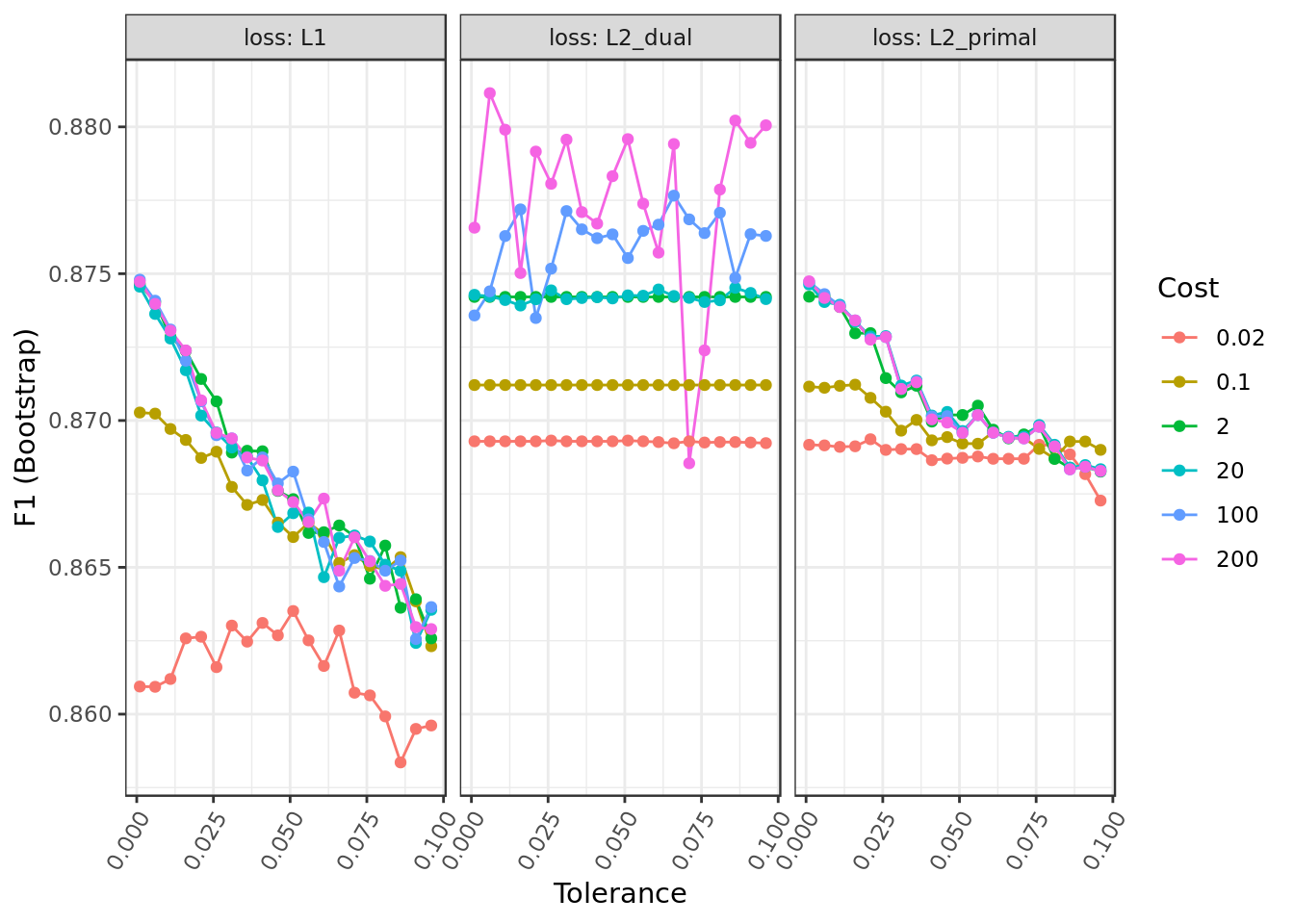

The hyper-parameter Loss seems to be the particularly meaningful for the Logistic Regression performance in this problem.

model.rl.smote %>%
  varImp() %$%
  importance %>%
  as.data.frame() %>%
  rownames_to_column(var="Feature") %>%
  mutate(Feature = tolower(Feature)) %>%
  ggplot() +
  geom_col(aes(x = reorder(Feature,eleito),y = eleito),
           position = position_dodge(width=0.8),width=0.6) + 
  labs(x="Feature", y="Overall Importance") +
  coord_flip()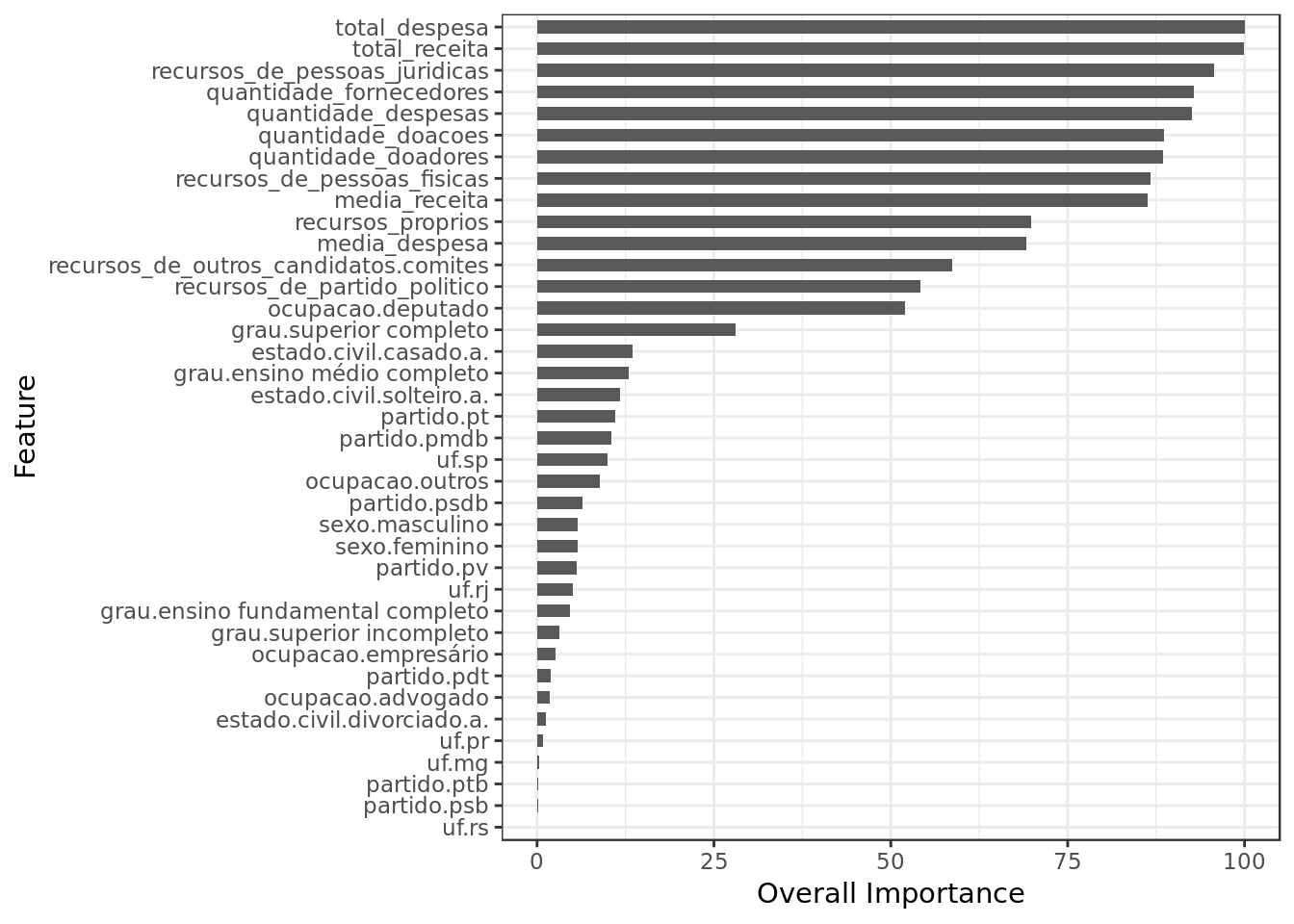

Total Receita (Total Revenue), Total Despesa (Total Expenditure) and Recursos de pessoas jurídicas (Revenue from Legal Entities) are together the three most important features in this model as well.
Despite regularization a lot of features were employed, however many were considered less important.

Quality metric

Train and Validation

model.rl.smote %$% 
  pred %>% 
  F_Measure(expected = .$obs,
            predicted = .$pred)

##      TP    TN   FP   FN    recall precision  accuracy f_measure
## 1 19486 27803 2137 3116 0.8621361 0.9011701 0.9000228  0.881221

The results in train/validation are overly optimistic in reason of the imbalance correction and should not be taken seriously.
Actual progress shall be assessed in the test stage

Test

test %>%
  select(-situacao) %>%
  predict(object=model.rl.smote,.) %>%
  F_Measure(test$situacao,.)

##    TP   TN  FP FN    recall precision  accuracy f_measure
## 1 172 1208 103 41 0.8075117 0.6254545 0.9055118  0.704918

We can see a substantial improvement compared with our previous attempt using Logistic Regression.

K nearest neighbours with SMOTE

neighborsGrid <- expand.grid(.k = seq(from=1, to=50, by=1))

oversampled %>%
  train(situacao ~ .,
        data = .,
        metric = "F1",
        method = "knn",
        na.action = na.omit,
        tuneGrid = neighborsGrid,
        trControl = trainControl(method = "boot",
                                 classProbs = TRUE,
                                 summaryFunction = f1,
                                 savePredictions = "final")) -> model.knn.smote

model.knn.smote

## k-Nearest Neighbors 
## 
## 5691 samples
##   38 predictors
##    2 classes: 'eleito', 'nao_eleito' 
## 
## No pre-processing
## Resampling: Bootstrapped (25 reps) 
## Summary of sample sizes: 5691, 5691, 5691, 5691, 5691, 5691, ... 
## Resampling results across tuning parameters:
## 
##   k   F1       
##    1  0.9400352
##    2  0.9210842
##    3  0.9112566
##    4  0.9039823
##    5  0.9027858
##    6  0.9017495
##    7  0.9021683
##    8  0.9018302
##    9  0.9029096
##   10  0.9019935
##   11  0.9035711
##   12  0.9030997
##   13  0.9030650
##   14  0.9028580
##   15  0.9020533
##   16  0.9012494
##   17  0.9009073
##   18  0.9002616
##   19  0.8993930
##   20  0.8989108
##   21  0.8973953
##   22  0.8971916
##   23  0.8968455
##   24  0.8961321
##   25  0.8955172
##   26  0.8951518
##   27  0.8951354
##   28  0.8951899
##   29  0.8950664
##   30  0.8944085
##   31  0.8941358
##   32  0.8945126
##   33  0.8941868
##   34  0.8937851
##   35  0.8931989
##   36  0.8930586
##   37  0.8928066
##   38  0.8923012
##   39  0.8917445
##   40  0.8920316
##   41  0.8914990
##   42  0.8915914
##   43  0.8916725
##   44  0.8912825
##   45  0.8910341
##   46  0.8907937
##   47  0.8906945
##   48  0.8903903
##   49  0.8902061
##   50  0.8895376
## 
## F1 was used to select the optimal model using the largest value.
## The final value used for the model was k = 1.

model.knn.smote %$%
  bestTune %$% 
  k -> bestParameter

model.knn.smote %$%
  results %>%
  ggplot(aes(k,F1)) +
  geom_vline(xintercept = bestParameter,
             color = "red") +
  geom_point(color="#0D98E8") +
  geom_line(color="#0D98E8") +
  labs(x="#Neighbors",
       y="F1 (Bootstrap)")

Our cross validation led to a knn with K=1, this may hint at a overfitting.

model.knn.smote %>%
  varImp() %$%
  importance %>%
  as.data.frame() %>%
  rownames_to_column(var="Feature") %>%
  mutate(Feature = tolower(Feature)) %>%
  ggplot() +
  geom_col(aes(x = reorder(Feature,eleito),y = eleito),
           position = position_dodge(width=0.8),width=0.6) + 
  labs(x="Feature", y="Overall Importance") +
  coord_flip()

Total Receita (Total Revenue), Total Despesa (Total Expenditure) and Recursos de pessoas jurídicas (Revenue from Legal Entities) are together the three most important features in this model as well.

Quality metric

Train and Validation

model.knn.smote %$% 
  pred %>% 
  F_Measure(expected = .$obs,
            predicted = .$pred)

##      TP    TN   FP  FN    recall precision  accuracy f_measure
## 1 21659 27938 1943 818 0.9636072 0.9176765 0.9472669 0.9400812

The results in train/validation are overly optimistic in reason of the imbalance correction and should not be taken seriously.
We have train/validation results incredibly good, in fact too good.
- This adds up to the hypothesis of a overfitting.

Test

test %>%
  select(-situacao) %>%
  predict(object=model.knn.smote,.) %>%
  F_Measure(test$situacao,.)

##    TP   TN  FP FN    recall precision  accuracy f_measure
## 1 168 1190 121 45 0.7887324 0.5813149 0.8910761 0.6693227

And here we have a steep decline in the test results, this is clear evidence that our KNN plus SMOTE overfitted.

Decision Tree with SMOTE

rpart.grid <- expand.grid(.cp = seq(from=0, to=0.1, by=0.005))

caret::train(x = select(oversampled, -situacao),
             y = oversampled$situacao,
             metric = "F1",
             method = "rpart",
             na.action = na.omit,
             tuneGrid = rpart.grid,
             trControl = trainControl(method = "boot",
                                      classProbs = TRUE,
                                      summaryFunction = f1,
                                      savePredictions = "final")) -> model.tree.smote

model.tree.smote

## CART 
## 
## 5691 samples
##   38 predictors
##    2 classes: 'eleito', 'nao_eleito' 
## 
## No pre-processing
## Resampling: Bootstrapped (25 reps) 
## Summary of sample sizes: 5691, 5691, 5691, 5691, 5691, 5691, ... 
## Resampling results across tuning parameters:
## 
##   cp     F1       
##   0.000  0.8899765
##   0.005  0.9000984
##   0.010  0.8988393
##   0.015  0.8984934
##   0.020  0.8984934
##   0.025  0.8984934
##   0.030  0.8984934
##   0.035  0.8984934
##   0.040  0.8984934
##   0.045  0.8984934
##   0.050  0.8984934
##   0.055  0.8984934
##   0.060  0.8984934
##   0.065  0.8984934
##   0.070  0.8984934
##   0.075  0.8984934
##   0.080  0.8984934
##   0.085  0.8984934
##   0.090  0.8984934
##   0.095  0.8984934
##   0.100  0.8984934
## 
## F1 was used to select the optimal model using the largest value.
## The final value used for the model was cp = 0.005.

model.tree.smote %$%
  bestTune %$% 
  cp -> bestParameter

model.tree.smote %$%
  results %>%
  ggplot(aes(cp,F1)) +
  geom_vline(xintercept = bestParameter,
             color = "red") +
  geom_point(color="#0D98E8") +
  geom_line(color="#0D98E8") +
  labs(x="Complexity Parameter",
       y="F1 (Bootstrap)")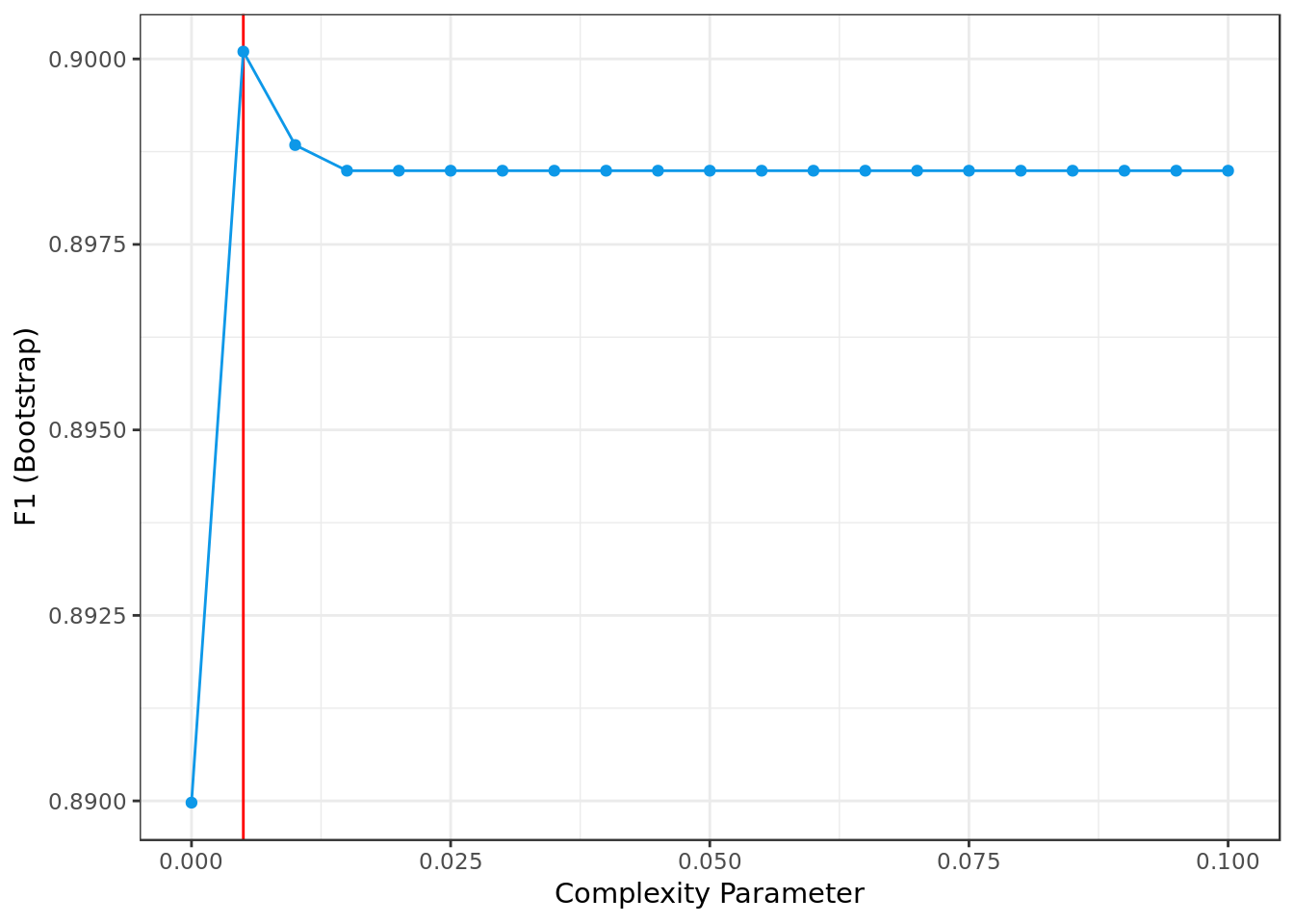

model.tree.smote %>%
  varImp() %$%
  importance %>%
  as.data.frame() %>%
  rownames_to_column(var="Feature") %>%
  mutate(Feature = tolower(Feature)) %>%
  ggplot() +
  geom_col(aes(x = reorder(Feature,Overall),y = Overall),
           position = position_dodge(width=0.8),width=0.6) + 
  labs(x="Feature", y="Overall Importance") +
  coord_flip()

Total Receita (Total Revenue), Total Despesa (Total Expenditure) and Recursos de pessoas jurídicas (Revenue from Legal Entities) are together the three most important features in this model as well.

model.tree.smote %$%
  finalModel %>%
  fancyRpartPlot(sub="")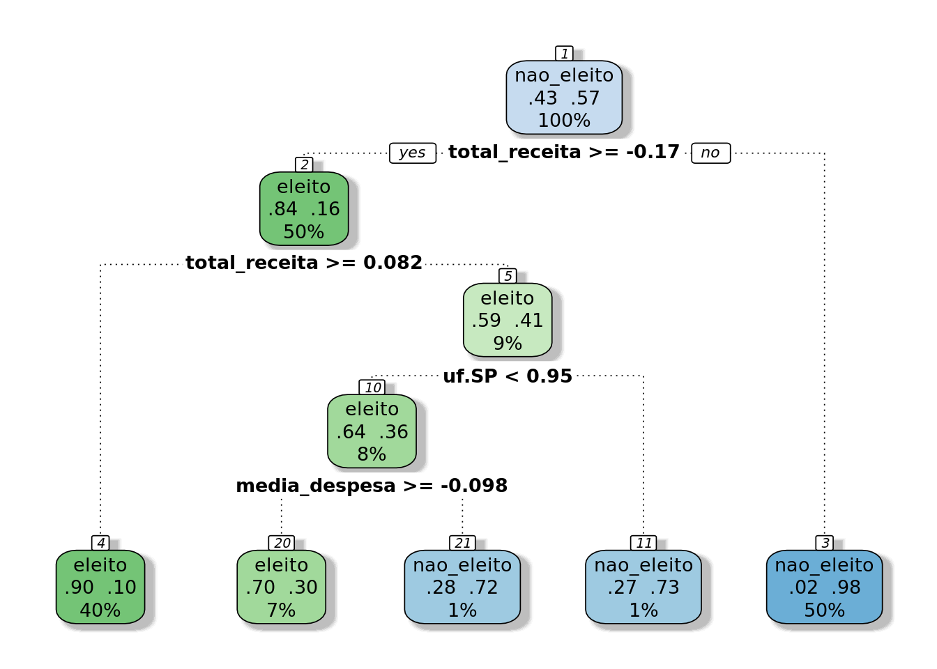

Here we have a tree of reasonable depth where the tree most important features have been integrated.

Quality metric

Train and Validation

model.tree.smote %$% 
  pred %>% 
  F_Measure(expected = .$obs,
            predicted = .$pred)

##      TP    TN   FP   FN    recall precision accuracy f_measure
## 1 21139 26432 3425 1263 0.9436211 0.8605683 0.910293 0.9001831

The results in train/validation are overly optimistic in reason of the imbalance correction and should not be taken seriously.

Test

test %>%
  select(-situacao) %>%
  predict(object=model.tree.smote,.) %>%
  F_Measure(test$situacao,.)

##    TP   TN  FP FN    recall precision  accuracy f_measure
## 1 198 1154 157 15 0.9295775 0.5577465 0.8871391 0.6971831

A result similar to that of the Logistic Regression plus SMOTE

AdaBoost with SMOTE

train(x = select(oversampled, -situacao),
      y = oversampled$situacao,
      metric = "F1",
      na.action = na.exclude,
      method='adaboost',
      tuneLength=2,
      trControl = trainControl(savePredictions = "final",
                               summaryFunction = f1,
                               classProbs = TRUE,
                               method = "boot")) -> model.ada.smote

model.ada.smote

## AdaBoost Classification Trees 
## 
## 5691 samples
##   38 predictors
##    2 classes: 'eleito', 'nao_eleito' 
## 
## No pre-processing
## Resampling: Bootstrapped (25 reps) 
## Summary of sample sizes: 5691, 5691, 5691, 5691, 5691, 5691, ... 
## Resampling results across tuning parameters:
## 
##   nIter  method         F1       
##    50    Adaboost.M1    0.9424543
##    50    Real adaboost  0.9427599
##   100    Adaboost.M1    0.9428177
##   100    Real adaboost  0.9434600
## 
## F1 was used to select the optimal model using the largest value.
## The final values used for the model were nIter = 100 and method =
##  Real adaboost.

model.ada.smote %$%
  results %>%
  ggplot(aes(nIter,F1, 
             color=as.factor(method))) +
  geom_point(shape=1) +
  geom_line() +
  labs(x="# Trees",y="F1 (Bootstrap)") +
  guides(color = guide_legend(title = "Method"))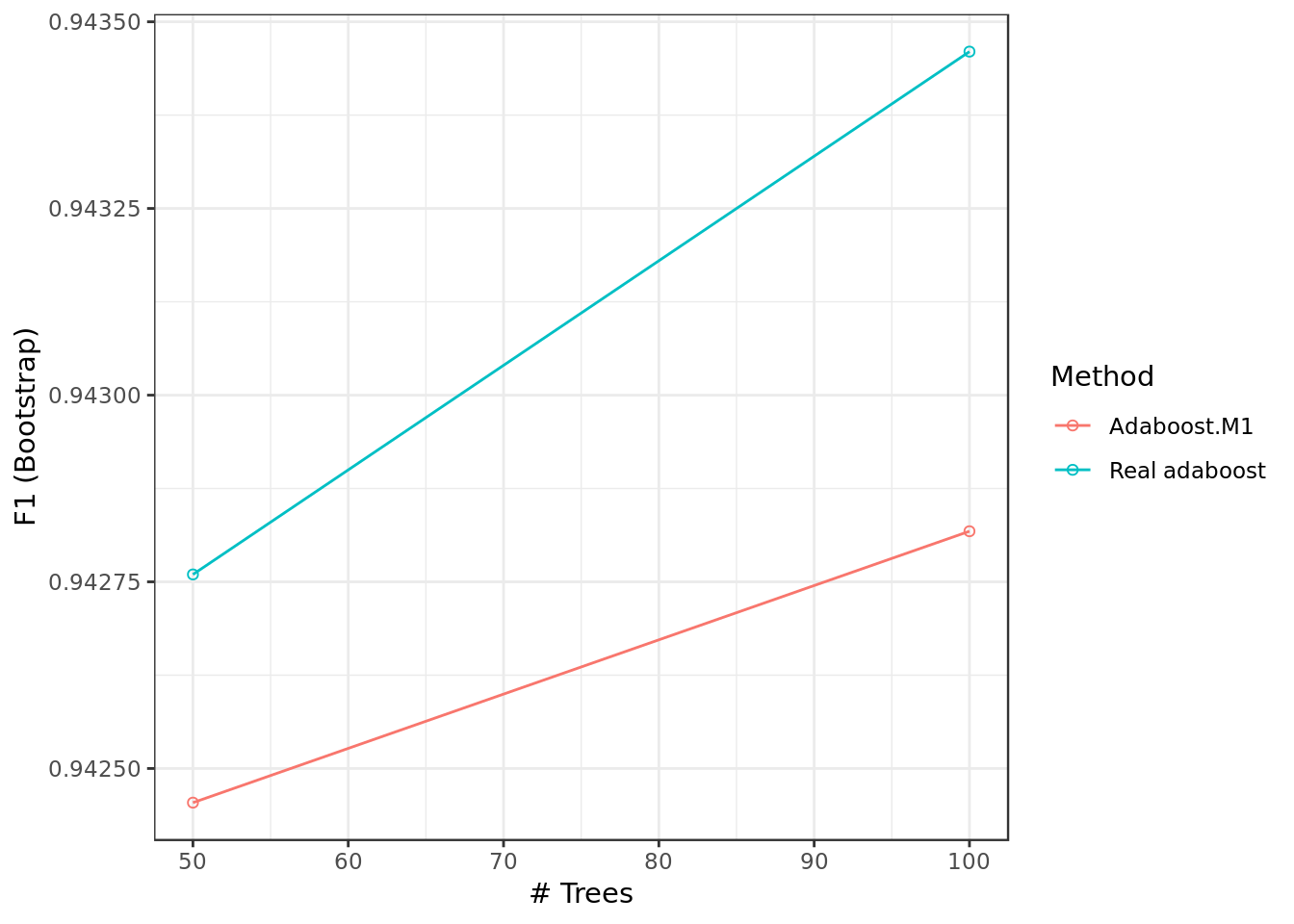

Quality metric

Train and Validation

model.ada.smote %$% 
  pred %>% 
  F_Measure(expected = .$obs,
            predicted = .$pred)

##      TP    TN   FP  FN    recall precision  accuracy f_measure
## 1 21949 27765 2011 621 0.9724856 0.9160684 0.9497192 0.9434343

The results in train/validation are overly optimistic in reason of the imbalance correction and should not be taken seriously.
Actual progress shall be assessed in the test stage

Test

test %>%
  select(-situacao) %>%
  predict(object=model.ada.smote,.) %>%
  F_Measure(test$situacao,.)

##    TP   TN  FP FN    recall precision accuracy f_measure
## 1 190 1173 138 23 0.8920188 0.5792683 0.894357  0.702403

Results similar to those of the Logistic Regression plus SMOTE

Classification of candidates in Brazilian elections

Introduction

Data Overview

The variables

Each item corresponds to a candidate, the attributes of each item are as follows:

Loading Data

Data Exploration

Imbalance on class distribution

There’s a strong imbalance in the class distribution of the dataset with around 13% of the entries in the class “eleito” (elected).

Preparing data

Splitting data

Scale and Center

One Hot Encoding

Train Shape

Observations: 6098

Variables: 263

Near Zero Variance Predictors

Unbalanced dataset

Logistic Regression

Quality metric

Train and Validation

Test

K nearest neighbours

Quality metric

Train and Validation

Test

Decision Tree

Quality metric

Train and Validation

Test

AdaBoost

Train and Validation

Test

Applying Oversample (SMOTE)

Logistic Regression with SMOTE

Quality metric

Train and Validation

Test

K nearest neighbours with SMOTE

Quality metric

Train and Validation

Test

Decision Tree with SMOTE

Quality metric

Train and Validation

Test

AdaBoost with SMOTE

Quality metric

Train and Validation

Test

Benardi Nunes

Classification of candidates in Brazilian elections

Analysis with Regularization on Brazilian elections

Analysis on Brazilian elections

C.E.A.P analysis (suppliers and weekend expenses)

C.E.A.P Analysis

Multivariate logistic regression on speed dating data

Multivariate linear regression on speed dating data

Analysis on MovieLens dataset with bootstrap

Analysis on Github commits (2016-2017)

Case Based Reasoning System for MSRP estimation