
Case Based Reasoning System for MSRP estimation
Introduction
Employed data, scripts and a brief description can be found at the original repository. Further references can be found at the page of Prof. Ian Watson.
library(FNN)
library(here)
library(magrittr)
library(tidyverse)

source(here::here("code/calc_KNN_error.R"))

theme_set(theme_bw())
Data Overview
Data has the following attributes:
Make: Make of the car;Model: Model of the car;Year: Manufacturing Date;Engine.Fuel.Type: Kind of fuel the engine runs on;Engine.HP: Engine HorsePower;Engine.Cylinders: Number of cylinders in the engine;Transmission.Type: Type of car transmission;Driven_Wheels: Wheels added;Number.of.Doors: Number of doors;Vehicle.Size: Vehycle size;Vehicle.Style: Vehycle style;highway.MPG: Miles per gallon on road;city.mpg: Miles per gallon on city;Popularity: Car popularity;MSRP: Manufacturer’s Suggested Retail Price and target variable.
Loading Data
read_csv(here::here("evidences/msrp.csv"),
         progress = FALSE,
         col_types =
           cols(
            Make = col_character(),
            Model = col_character(),
            Year = col_integer(),
            `Engine Fuel Type` = col_character(),
            `Engine HP` = col_integer(),
            `Engine Cylinders` = col_integer(),
            `Transmission Type` = col_character(),
            Driven_Wheels = col_character(),
            `Number of Doors` = col_integer(),
            `Market Category` = col_character(),
            `Vehicle Size` = col_character(),
            `Vehicle Style` = col_character(),
            `highway MPG` = col_integer(),
            `city mpg` = col_integer(),
            Popularity = col_integer(),
            MSRP = col_integer()
            )) %>%
  drop_na() -> car_data
Dummify Categorical Variables
car_data %>%
  mutate(
    Make = as.numeric(factor(Make)),
    Model = as.numeric(factor(Model)),
    `Engine Fuel Type` = as.numeric(factor(`Engine Fuel Type`)),
    `Transmission Type` = as.numeric(factor(`Transmission Type`)),
    Driven_Wheels = as.numeric(factor(Driven_Wheels)),
    `Market Category` = as.numeric(factor(`Market Category`)),
    `Vehicle Size` = as.numeric(factor(`Vehicle Size`)),
    `Vehicle Style` = as.numeric(factor(`Vehicle Style`)))-> car_data

car_data %>%
    glimpse()
## Observations: 11,812
## Variables: 16
## $ Make <dbl> 6, 6, 6, 6, 6, 6, 6, 6, 6, 6, 6, 6, 6, 6, 6,…
## $ Model <dbl> 5, 4, 4, 4, 4, 4, 4, 4, 4, 4, 4, 4, 4, 4, 4,…
## $ Year <int> 2011, 2011, 2011, 2011, 2011, 2012, 2012, 20…
## $ `Engine Fuel Type` <dbl> 8, 8, 8, 8, 8, 8, 8, 8, 8, 8, 8, 8, 8, 8, 8,…
## $ `Engine HP` <int> 335, 300, 300, 230, 230, 230, 300, 300, 230,…
## $ `Engine Cylinders` <int> 6, 6, 6, 6, 6, 6, 6, 6, 6, 6, 6, 6, 6, 6, 6,…
## $ `Transmission Type` <dbl> 4, 4, 4, 4, 4, 4, 4, 4, 4, 4, 4, 4, 4, 4, 4,…
## $ Driven_Wheels <dbl> 4, 4, 4, 4, 4, 4, 4, 4, 4, 4, 4, 4, 4, 4, 4,…
## $ `Number of Doors` <int> 2, 2, 2, 2, 2, 2, 2, 2, 2, 2, 2, 2, 2, 2, 2,…
## $ `Market Category` <dbl> 38, 67, 64, 67, 63, 67, 67, 64, 63, 63, 64, …
## $ `Vehicle Size` <dbl> 1, 1, 1, 1, 1, 1, 1, 1, 1, 1, 1, 1, 1, 1, 1,…
## $ `Vehicle Style` <dbl> 9, 7, 9, 9, 7, 9, 7, 9, 7, 7, 9, 9, 7, 7, 9,…
## $ `highway MPG` <int> 26, 28, 28, 28, 28, 28, 26, 28, 28, 27, 28, …
## $ `city mpg` <int> 19, 19, 20, 18, 18, 18, 17, 20, 18, 18, 20, …
## $ Popularity <int> 3916, 3916, 3916, 3916, 3916, 3916, 3916, 39…
## $ MSRP <int> 46135, 40650, 36350, 29450, 34500, 31200, 44…Checking for missing values
row.has.na <- apply(car_data,
                    1,
                    function(x){any(is.na(x))})
noquote(paste('Number of rows with misssing values: ',
            sum(row.has.na)))
## [1] Number of rows with misssing values: 0Applying scale to predictor variables
num.vars <- sapply(car_data,
                   is.numeric,
                   simplify=F)

num.vars$MSRP = FALSE
num.vars <- unlist(num.vars)

car_data[num.vars] <- lapply(car_data[num.vars],
                             scale)
car_data %>%
  sample_n(10)
## # A tibble: 10 x 16
## Make[,1] Model[,1] Year[,1] `Engine Fuel Ty… `Engine HP`[,1]
## <dbl> <dbl> <dbl> <dbl> <dbl>
## 1 0.556 -0.959 0.347 -0.0820 3.40
## 2 1.54 1.29 0.874 -0.755 -0.453
## 3 1.54 1.31 0.742 -4.79 -0.0870
## 4 1.47 1.47 0.611 0.591 -0.627
## 5 1.54 0.827 -0.0476 0.591 0.0137
## 6 0.906 0.354 -0.838 0.591 -0.591
## 7 -0.984 1.35 0.874 0.591 0.353
## 8 0.416 -0.760 0.742 0.591 -0.600
## 9 -0.634 -0.445 0.742 0.591 0.691
## 10 -0.984 1.05 0.874 -2.10 0.325
## # … with 11 more variables: `Engine Cylinders`[,1] <dbl>, `Transmission
## # Type`[,1] <dbl>, Driven_Wheels[,1] <dbl>, `Number of Doors`[,1] <dbl>,
## # `Market Category`[,1] <dbl>, `Vehicle Size`[,1] <dbl>, `Vehicle
## # Style`[,1] <dbl>, `highway MPG`[,1] <dbl>, `city mpg`[,1] <dbl>,
## # Popularity[,1] <dbl>, MSRP <int>Validation
Split data into training/testing sets
set.seed(101)

## Adding surrogate key to dataframe
car_data$id <- 1:nrow(car_data)

car_data %>%
  dplyr::sample_frac(.8) -> train

dplyr::anti_join(car_data,
                 train,
                 by = 'id') -> test
Dissociate predictors from target variable/surrogate key
train %>%
  select(-MSRP,-id) -> train.predictors

train %>%
  select(MSRP, id) -> train.response

test %>%
  select(-MSRP,-id) -> test.predictors

test %>%
  select(MSRP, id) -> test.response
Apply K Nearest Neighbor
Calculate accumulated error
results <- data.frame(matrix(ncol = 0, nrow = 10))
results$k <- seq(1,10,1)

accum_err <- c()

for(num in results$k) {

  calc_KNN_error(num,
         train.predictors,
         test.predictors,
         train$id,
         train.response,
         test.response) -> err

  accum_err <-c(accum_err, err)
}

results$accum_err <- accum_err

results
## k accum_err
## 1 1 4.043619e+11
## 2 2 1.370266e+12
## 3 3 1.051143e+12
## 4 4 1.664537e+12
## 5 5 2.180589e+12
## 6 6 2.517307e+12
## 7 7 2.853242e+12
## 8 8 3.129612e+12
## 9 9 3.263991e+12
## 10 10 3.361216e+12results %>%
ggplot(aes(k,accum_err)) +
geom_point(size = 3,
alpha = .6) +
geom_line() +
scale_x_continuous(breaks=seq(1,10,1)) +
labs(y="Accumulated Error", x= "K Value") +
ggtitle("Accumulated Error by K value")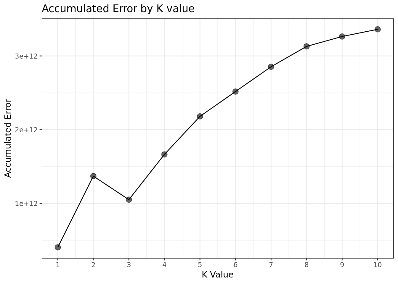
Results
- A smaller K seems to render less accumulated error.
- At K = 2, we have an unusual spike in terms of accumulated error, which one could impute on a probable overfit.
- K = 1 renders the smallest amount of Accumulated Error.

